Dear Allpix Developers,
I am currently working with Allpix^2 for the first time and I’m having some issues with the implementation of multiplication module.
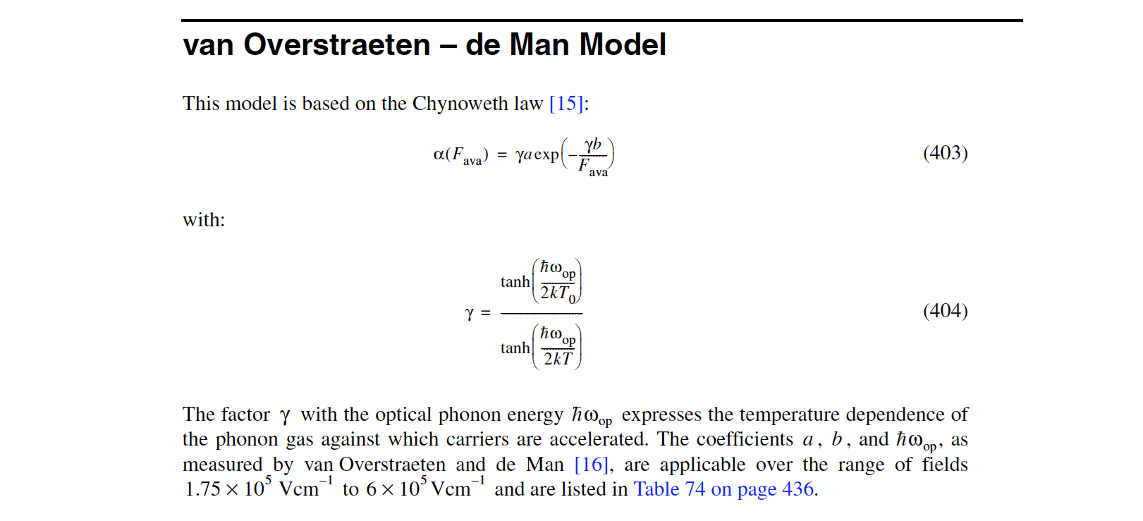
In particular, I’m trying to implement a simulation with a 2D electric field map provided by TCAD of a monolithic sensor with a gain layer. I’m using the Van Overstraeten-De Man Model in the TransientPropagation module as follows:
[TransientPropagation]
log_level = DEBUG
temperature = 300K
charge_per_step = 4
timestep = 1ps
integration_time = 20ns
induction_matrix = 1, 1
output_plots = true
timestep_max = 0.005ns
multiplication_model = "overstraeten"
multiplication_threshold = 300kV/cm
To estimate the gain of the detector, I repeated the same simulation removing the last two lines above.
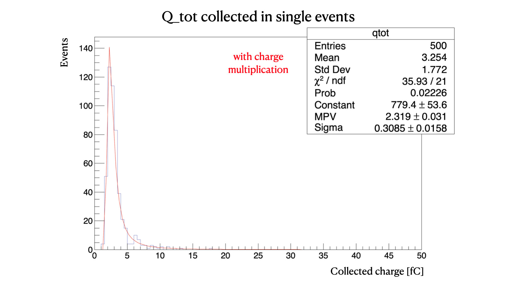
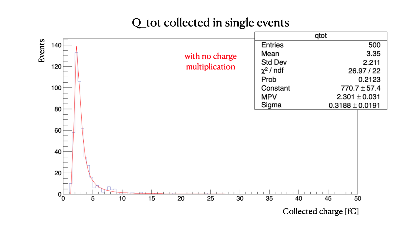
At this point for both the cases, I calculated the total charge collected in every single events and I represented it in a histogram. Fitting the distributions with a landau, I can extract the gain value as the ratio of the two MPV values from the fits.
However as you can notice in the figures, the two distributions and MPVs are similar and it seems the multiplication module isn’t active.
Could someone help me to understand this problem?
Thanks a lot,
Giulia
Ciao @ggioachi,
Your configuration looks fine, but the result indeed indicates that there was no charge multiplication happening. Would you mind checking if your electric field indeed exceeds the threshold field of 300kV/cm at any position in the sensor?
Simon
Dear @simonspa,
thanks for your reply.
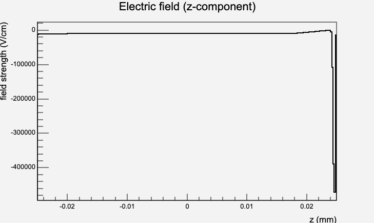
The electric field exceeds the value of 300kV/cm near the gain layer but away from it the value is smaller, as you can see in the following figure.
Nevertheless I tried to change the threshold using values from 0kV/cm to 300kV/cm, but the result is always the same.
Do you have other suggestions?
Thanks again,
Giulia
Hi @ggioachi
your field indeed looks fine -may I ask which version of Allpix Squared you are using? The output of
allpix --version
should help here. Also, could you run a few events with
allpix -c your_config.conf -o TransientPropagation.log_level=DEBUG -o number_of_events=5
so we can see what’s going on?
Thanks,
Simon
Dear @ggioachi
In addition, it would be helpful if you could provide also the rest of the configuration file - then we could have a look whether the issue is located in another module.
Cheers
Paul
Dear @simonspa and @pschutze,
thanks again for your reply.
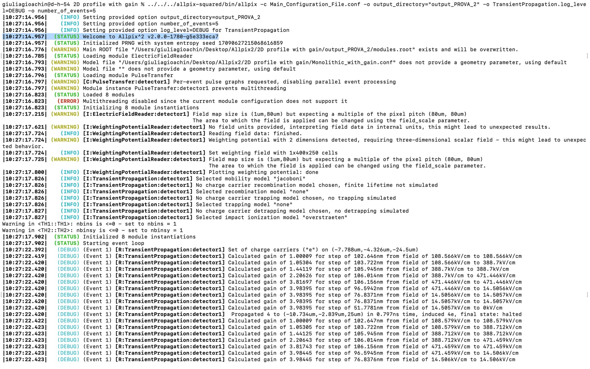
I send you the first lines of my terminal when I run the simulation as you request:
I highlighted the version of Allpix Squared I’m using.
As I already noticed, it seems there is a gain during the simulation (which value is always between 1 and 4, even if we expect a gain of 15 based on the doping of our gain layer) but then when I calculate the ratio between the MPVs the gain results equal to 1.
Moreover, when I run the simulation without the multiplication model, I find a gain value of 1 written on my terminal as expected.
As request, I send you my configuration file:
Main_Configuration_File.conf (3.4 KB)
Thank you very much for your help,
Giulia
Dear @ggioachi ,
thanks a lot! Indeed I have the fear that we’re not treating the gain correctly in the TransientPropagation module. I will have a close look at this in the coming days.
In the meantime, if you would like to perform a cross-check, you could run the simulation using the GenericPropagation module using equivalent parameters and check, whether the gain is correctly represented therein.
Concerning the gain: you could still try to further reduce the time step, as currently you do “only” 4-5 steps within the multiplication region.
Cheers
Paul
Dear @ggioachi ,
We’re looking into this and are currently discussing the behaviour.
I did a couple of tests myself and I have the following suggestions/questions for you:
- The timesteps you are using (
timestep_min = 1ps and timestep_max = 5ps) are quite large. Please try reducing the maximum timestep to 1ps or even less. A good approach is typically to start with a high value and reduce it for as long as you see a change. I would assume this brings you to around a picosecond or less.
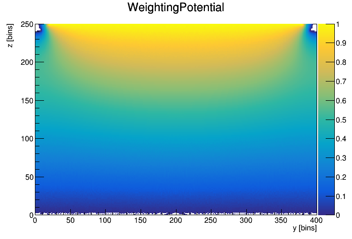
- Do you have a graph at hand representing the weighting potential in your sensor?
Cheers
Paul
Dear @pschutze,
thank you very much for your suggestions and your help!
- I tried to run the simulation using the
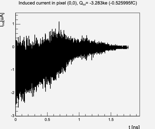
GenericPropagation module and using equivalent parameters. Thanks to the log_level = DEBUG, I measured some gain but I obtained strange waveforms of the induced current (as the one I attach you).
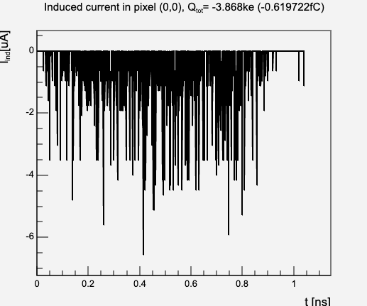
Therefore, does the GenericPropagation module take into account the weighting potential for calculate the induced charge via the Shockley-Ramo theorem?
- Then, as you suggested, I tried to reduce the time step in the
TransientPropagation module. In this module I couldn’t use the parameters timestep_min and timestep_max, but only timestep.
Nevertheless I ran a simulation reducing the timestep and using these parameters:
[TransientPropagation]
#log_level = DEBUG
temperature = 300K
charge_per_step = 4
timestep = 0.1ps
integration_time = 20ns
induction_matrix = 1, 1
output_plots = true
multiplication_model = “overstraeten”
multiplication_threshold = 300kV/cm
In the terminal I could find a mean gain slightly bigger (around 5) and the steps within the multiplication region are grown. However, I obtained noisy signals respect to the previous simulation. Is this an effect of the timestep reduction?
- Finally, I send you the graph of the weighting potential in my sensor as you requested. Until now I have simulated a matrix with only 1 pixel.
Thanks again,
Giulia
Hi @ggioachi ,
thank you for coming back to us!
Concerning the GenericPropagation: this module does not use the Shockley-Ramo theorem but when trying to extract pulses, the time of the collection of the individual charge carriers is used as pulse information. This is of course an approximation which in case of impact ionisation does not hold true at all. I was only interested in the gain that is reached (there’s also the gain_histo graph, which shows the distribution of amplification numbers).
Now, more important, the TransientPropagation: I am sorry to say that we have (thanks to this thread!) identified quite a flaw in our simulation. Right now, we do induce a larger current when a charge carrier sees a gain, which is equivalent to the generation of same-type charge carriers. However, we lack the generation of opposite-type charge carriers and their propagation in the sensor. In other words, and for most cases: an electron generates more electrons, but no holes. This is of course unphysical and by far not insignificant for LGADs or alike.
We have addressed this immediately and filed the following merge request:
It might still take a bit until this is released, as we still have to figure out a few details. And although this is not final, I would invite you to test the code and see whether it matches your expectations more than the current version.
If you are willing to try this but need hints on how to fetch and install this, please let us know!
Cheers
Paul
Hi @pschutze,
thanks a lot for your help! 
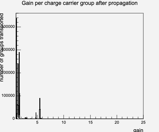
I send you this graph in order to have an idea of the gain using the GenericPropagation module.
Concerning TransientPropagation, I’m happy you have found a possible cause to my issue! Now I will test the new code and give you my feedback.
However, I have recently begun my PhD and I don’t know how to use GitLab very well.
Could you help me to fetch and install this current version?
Thank you very much,
Giulia
Hi @ggioachi ,
it looks like the gain is still not quite what you would expect from what you mentioned earlier on. However, keep in mind that the graph you showed (thanks!) represents the number of charge carriers created per individual charge carrier. Hence, it is connected to the induced charge, but it’s certainly not a 1:1 representation. Hence, the TransientPropagation will be needed for you to evaluate this number better.
To fetch and install the latest version: in what way are you running Allpix Squared? Did you install it yourself or are you running it via CVMFS or docker?
If you’re running a local installation, simply do the following:
- Navigate to your Allpix Squared directory
-
git fetch origin (if you got the code from somewhere else than our main repository, you’d need to change that, but probably this is not the case)
git checkout -b fix_induction_gain fix_induction_gain- Then re-install by moving to the build directory and compiling the code:
I hope this works for you. If it doesn’t, please let us know a few more details.
Cheers
Paul
Hi @pschutze,
thank you very much!
Now I try to install it and I will write you as soon as possible for any news 
Thanks again,
Giulia
Ciao @ggioachi
the code in fix_induction_gain should now be final to what will be merged to the master branch. Please let us know if this works for you as expected!
Cheers,
Simon
Dear @simonspa,
thank you very much for your time spent helping me with the issue
In the past few days, I tried to run different simulations with your first version of the new code. Something seemed to be changed, but I still obtained a gain value smaller than expected.
Now I try this new version and let you know my feedback as soon as possible!
Thank you again,
Giulia
Dear @simonspa and @pschutze,
I ran the simulation using the last version of the code. Unfortunately, I don’t obtain yet the results I expected.
I continue to find a gain of the order of 4 (when I use the Overstraeten model) and 6 (trying the Okuto model), which are very different from the expected gain value of 15-20.
I sent you a waveform of the induced current obtained using the Okuto model.
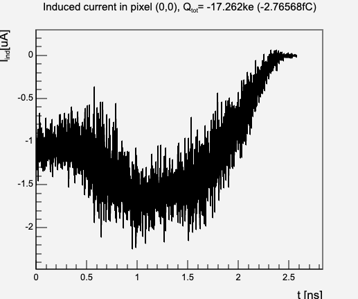
Its trend is similar to the expected one, with a second “peak” higher than the first. However, the maximum value reached is smaller by a factor of 3-4.
In conclusion, I noticed a change with the first version of the code (where there wasn’t the holes multiplication) because now the current signals are different with or without the multiplication model. However, I didn’t see the difference between the first and the last version of the code I tested.
Even if the current trend with the Okuto model seems similar to the one expected from the TCAD simulation, I continue to obtain a small gain.
Could you help me again with this issue?
Thank you very much,
Giulia
Dear @ggioachi ,
thank you very much for reporting back.
For your information: with the last commits that you probably checked out, we did not change much in the functionality for LGAD sensors rather than fixed potential scenarios that would break the simulation.
However, on the general comment that the read out charge is lower than the expected one, this of course remains a bit puzzling. Can you comment on what you are comparing this to, so where the expected gain of 15 is coming from?
Cheers
Paul
Dear @pschutze,
thanks for your explanation!
The expected gain was obtained as the ratio of a simulation with impact ionization enabled and one without it, using the Overstraeten model.
This simulation was repeated using the Garfield++ tool, where we found a gain of 15, and using TCAD, where we obtained almost 20. Now, we wanted to repeat it using Allpix Squared.
We would like to investigate the difference found with the different simulation tools.
Thanks for your help,
Giulia
Dear @pschutze,
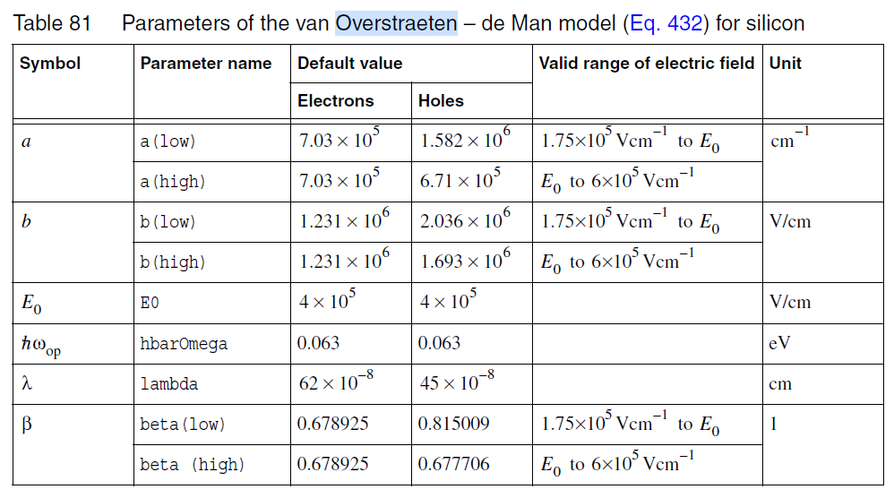
I was reading the TCAD manual to understand how it calculates the gain with the Overstraeten model when I noticed that one parameter (called hbarOmega) is different by a factor of 10^6 compared to the one in Allpix Squared.
Could this difference explain the divergence between the two tools’ results?
I post below the impact ionization coefficient according to the TCAD tool and the table with the parameters.
Thank you again,
Giulia
Hi @ggioachi ,
thank you very much for you help. The latest updates that you tested are now merged to the master branch. However, we’re still trying to find out what is causing the large difference in the results.
Indeed, there was a typo with the hbarOmega, which will be fixed. However, this doesn’t change too much in the result, if the temperature is set around room temperature (at 300 K the error is cancelling out, and the result remains the same).
Cheers
Paul