Charge collection efficiency using DepositionPointCharge in irradiated detector

simonspa · April 21, 2023, 4:27pm

Thanks for running these, quite interesting. My naive thought was that the combination GP+IT would be very similar to what e.g. pixel av does.

When we use the latter config, the CCE is low by ~0.2% at every Z deposition position.

Rather 20% I would say - which is interesting and certainly wrong! I have to admit that the IT module has not been battle-tested a lot because I wrote it essentially for your exact use case - but nobody had worked in that yet.

Also, the very odd shape coming from the TP+IT combination should not happen of course, we have to correctly catch that there is already pulse information available. I will look into this…

Simon

simonspa · April 21, 2023, 5:47pm

Hi @knakkali

just to confirm - are you still on v2.3.2? Would you mind testing this on the current master instead? I noticed a significant difference in an algorithm relevant for your simulation…

This is what you need to change in your config:

[ElectricFieldReader]
# Add this:
field_mapping = SENSOR

[WeightingPotentialReader]
# Add this:
field_mapping = PIXEL_FULL

[TransientPropagation]
# replace induction_matrix with this:
distance = 1

You can e.g. use the latest version deployed to CVMFS if you were using the tagged version from there before.

Cheers,
Simon

simonspa · April 24, 2023, 4:30pm

Hi @knakkali

some more things to try out: @pschutze reminded me that the valid-looking results from your early posts were performed on Pixel (0,0) while the later results that look significantly different come from the sensor center.

To check if there is any difference with respect to the border pixels that affects the result, you could try running with

[TransientPropagation]
induction_matrix = 1, 1

to only calculate the induced current under the central pixel (should be enough for your purposes). For master this corresponds to setting distance = 0.

With this, a comparison between pixel 0,0 and the center of a pixel somewhere in the matrix would be interesting.

Cheers,
Simon

knakkali · April 25, 2023, 9:32am

Hello @simonspa ,

Thanks a lot for your reply. Here are the CCE vs Z results in master and v2.3.3:

The screenshot on the left shows the CCE vs Z using TP+PT and GP+IT in v2.3.3 (left fig) and latest(right fig). In the master, the differences are now about 2% while it us 20% in v2.3.3 (I got the numbers correct this time )

The screenshot on the right shows CCE vs Z results while using TP+IT in v2.3.3 and latest. Here we have the exact;y same odd CCE vs Z shape.

Thanks a lot,
Keerthi

knakkali · April 25, 2023, 12:59pm

Hello @simonspa and @pschutze

Here are the results of comparison of CCE vs Z for Qinj = 0,0,Z and Qinj = 10mm,4.8mm,Z with distance =0 using GP+IT and TP+PT

Pixel 00 seems to be special

Cheers
@mbomben and Keerthi

simonspa · April 26, 2023, 8:43pm

Hi @knakkali

thanks for these results, very very interesting. I’ll do some cross-checks in the coming days, I’m very curious where this could come from. Could you - for reference - again attach the relevant configs here? Just to make sure I have your most up-to-date versions…

Re: the weird share with TP+IT: this is expected since we’re already having a pulse with induced current from TP, and are then suddenly adding on top yet another induced current from IT. So this is double counting in a very odd way. I have now added code that prevents IT from running when there is pulse information already available.

Cheers,
Simon

knakkali · April 27, 2023, 8:57am

Hello @simonspa ,

Thank you so much for the explanation of TP+IT weird shape. I can now see why this happens.

Here are my latest configs: CERNBox

Cheers
Keerthi

simonspa · May 9, 2023, 2:33pm

Hi @knakkali

I had a look at your example and I found the reason for the difference. It is however, not a bug in the code per say, but a logical result of how we do the simulation.

First, have a look at the output of the PulseTransfer for a single event, once in the corner of the sensor and once in the center:

With Trapping

Pixel (0,0)

(D) (E: 1) [R:PulseTransfer:detector1] Pixel (0,0) has charge of -821e with 200 ancestors
(D) (E: 1) [R:PulseTransfer:detector1] Pixel (0,1) has charge of 37e with 200 ancestors
(D) (E: 1) [R:PulseTransfer:detector1] Pixel (1,0) has charge of 37e with 200 ancestors
(D) (E: 1) [R:PulseTransfer:detector1] Pixel (1,1) has charge of 21e with 200 ancestors
(I) (E: 1) [R:PulseTransfer:detector1] Total charge induced on all pixels: -726e

Pixel (200,96)

(D) (E: 1) [R:PulseTransfer:detector1] Pixel (199,95) has charge of 21e with 200 ancestors
(D) (E: 1) [R:PulseTransfer:detector1] Pixel (199,96) has charge of 36e with 200 ancestors
(D) (E: 1) [R:PulseTransfer:detector1] Pixel (199,97) has charge of 21e with 200 ancestors
(D) (E: 1) [R:PulseTransfer:detector1] Pixel (200,95) has charge of 37e with 200 ancestors
(D) (E: 1) [R:PulseTransfer:detector1] Pixel (200,96) has charge of -821e with 200 ancestors
(D) (E: 1) [R:PulseTransfer:detector1] Pixel (200,97) has charge of 37e with 200 ancestors
(D) (E: 1) [R:PulseTransfer:detector1] Pixel (201,95) has charge of 22e with 200 ancestors
(D) (E: 1) [R:PulseTransfer:detector1] Pixel (201,96) has charge of 37e with 200 ancestors
(D) (E: 1) [R:PulseTransfer:detector1] Pixel (201,97) has charge of 21e with 200 ancestors
(I) (E: 1) [R:PulseTransfer:detector1] Total charge induced on all pixels: -588e

Analysis

If you compare the central pixel, both see exactly the same charge, i.e. -821e. Neighbors see a non-zero charge being induced because of the imbalance between electrons and holes introduced by the trapping. I.e. if the hole gets trapped on its way to the backside, this induced charge does not go back to zero as it does when disabling trapping (see below).

However, for the corner pixel, there are only three neighbors (top, right, top-right) while for the central pixel there are eight neighboring pixels. Hence, if you simply calculate the sum of them all, you will get a lower total induced charge for the central pixel - only because you also count the neighbor pixels with a wrong-polarity induced current. Something that you probably don’t want to do…

Without Trapping

You can see the situation quite clearly when disabling trapping (just comment out the trapping_model parameter):

Pixel (0,0)

(D) (E: 1) [R:PulseTransfer:detector1] Pixel (0,0) has charge of -999e with 200 ancestors
(D) (E: 1) [R:PulseTransfer:detector1] Pixel (0,1) has charge of 1e with 200 ancestors
(D) (E: 1) [R:PulseTransfer:detector1] Pixel (1,0) has charge of 1e with 200 ancestors
(D) (E: 1) [R:PulseTransfer:detector1] Pixel (1,1) has charge of 0e with 200 ancestors
(I) (E: 1) [R:PulseTransfer:detector1] Total charge induced on all pixels: -997e

Pixel (200,96)

(D) (E: 1) [R:PulseTransfer:detector1] Pixel (199,95) has charge of 0e with 200 ancestors
(D) (E: 1) [R:PulseTransfer:detector1] Pixel (199,96) has charge of 1e with 200 ancestors
(D) (E: 1) [R:PulseTransfer:detector1] Pixel (199,97) has charge of 0e with 200 ancestors
(D) (E: 1) [R:PulseTransfer:detector1] Pixel (200,95) has charge of 1e with 200 ancestors
(D) (E: 1) [R:PulseTransfer:detector1] Pixel (200,96) has charge of -999e with 200 ancestors
(D) (E: 1) [R:PulseTransfer:detector1] Pixel (200,97) has charge of 1e with 200 ancestors
(D) (E: 1) [R:PulseTransfer:detector1] Pixel (201,95) has charge of 0e with 200 ancestors
(D) (E: 1) [R:PulseTransfer:detector1] Pixel (201,96) has charge of 1e with 200 ancestors
(D) (E: 1) [R:PulseTransfer:detector1] Pixel (201,97) has charge of 0e with 200 ancestors
(I) (E: 1) [R:PulseTransfer:detector1] Total charge induced on all pixels: -995e

Analysis

Here you not only see that we induce the full deposited 1000e, but also that the accumulated (final) charge induced in the neighbor pixels sums to zero (or 1e because of numerical precision).

Where To Go From Here

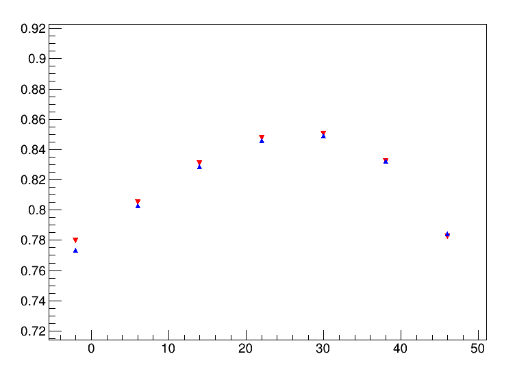
By simply only summing the PixelCharge contributions with the correct sign (and ignoring the others) I get a curve (red) that is very very close to the weighted CCE approach you have presented above (blue):

I would argue that this is a physically logical thing to do because your front-end will not detect these pulses. Alternatively, you could analyze the PixelHit object instead of the PixelCharge because there these neighbors have been suppressed, being below the threshold.

An alternative that would also save you computing time is to use distance = 0 and only calculate charge induced in the central pixel, and none of the neighbors. With the pitch and weighting field you have, you don’t expect a significant contribution from induction in neighbors anyway (small inter-pixel capacitance).

Our Homework

Currently, in the DefaultDigitizer we simply std::abs() the charge we get from the PixelCharge object - which in this case obviously is problematic. Not really problematic in your case, because 40e will certainly not cross your threshold, but still this is an improper treatment of the input data and we likely have to add a parameter to define the threshold polarity. Tracked here: DefaultDigitizer: Threshold Polarity (#273) · Issues · Allpix Squared / Allpix Squared · GitLab

With this,

happy simulation!

Simon

simonspa · May 10, 2023, 10:56am

Just to add to this: this is a physical effect nicely measured e.g. by Carolin Niemeyer in her thesis: Edge-on Measurements on Planar Pixel Sensors for the CMS Phase 2 Upgrade | ediss.sub.hamburg

Page 137 has this plot:

You can see that neighbor pixels in an irradiated sensor indeed do see these correctly simulated opposite-sign net charges.

simonspa · May 10, 2023, 3:00pm

@knakkali @mbomben

the difference is also nicely seen by comparing the same event, same pixel, same pulse once with and once without trapping: electron contribution at the beginning is the same, but hole induction is reduced by them getting trapped:

(red: cmstracker trapping, blue: no trapping)

Cheers,
Simon

knakkali · May 15, 2023, 10:44am

Hello @simonspa

Thank you so much for this very detailed explanation. I apologize for my delayed response. Last week was quite overwhelming due to the ITk week, and more importantly, we wanted to take the time to fully comprehend your answers.

We now have a clear understanding of the distinction between pixel (0,0) and pixel (200,96). Your suggestion of summing the pixel charge contributions with the correct sign works like a charm. we have made the necessary modifications to our analysis script, and here are the updated results:

The blue full dots represent the case where we summed the contribution of the central pixel and its neighbors (initial result) to calculate the induced charge. The red closed dots is the workaround method estimating induced charge using Ramo. Lastly, the blue open dots correspond to the case where we estimate induced charge based on the smallest pixel charge (eg: -821e )

Thanks a lot to you and @pschutze for helping us with this and all the interesting discussions we’ve had here.

Cheers,
@mbomben and Keerthi

simonspa · May 15, 2023, 11:02am

Hi @knakkali

that’s very nice to hear - physics is restored, the world is saved!

One small comment:

I would not calculate this like that. If you actually have charge sharing, you might as well get two or more pixels with correct charge induced. Just make sure you are only summing the charges with the sign that you expect (i.e. negative when collecting electrons). That should be safer than taking the maximum bin only.

Also, it would be great if you could cross-check with the GP+IT combination - that should be the most appropriate one for your studies, since you are not really interested in the timing behavior of the pulses, it might give you some computational advantage.

Cheers,
Simon

knakkali · May 15, 2023, 11:19am

Hello Simon,

I would not calculate this like that. If you actually have charge sharing, you might as well get two or more pixels with correct charge induced. Just make sure you are only summing the charges with the sign that you expect (i.e. negative when collecting electrons). That should be safer than taking the maximum bin only.

I kind of realised this while drafting my message to reply back to you that picking up the correct sign would be more accurate than looking for the smallest charge. Thanks for this comment. I’ll modify my code accordingly.

Also, will redo the simulations with GP+IT.

Cheers,
Keerthi