Using custom electric field

[asantra]

Hello,
I am trying to use custom electric field in Allpix2. Here is the relevant part of the config file:

[ElectricFieldReader]
model = "custom"
field_function = "[0]*x/(x*x+y*y+z*z)^(1.5)", "[0]*y/(x*x+y*y+z*z)^(1.5)", "[0]*z/(x*x+y*y+z*z)^(1.5)"
field_parameters = 12500V/cm, 12500V/cm, 12500V/cm
depletion_depth = 20um
output_plots = 1

I am looking at the electric field plots in the modules.root file. While I see the Z component of the electric field is 0 at z=0 (which is expected),

I see that Y component of the electric field is not 0 at y=0. In fact, I do not see any position dependence of the y component of the electric field.

What is going wrong here? Am I missing something?

Many thanks,
Arka

[pschutze]

Hi @asantra ,

one thing I’m spotting is, that the field_function is only evaluated in the region starting from the sensor surface down to the depletion depth. Hence, the field in your sensors here spans from 0.0125 to -0.0075, so that’s 20 micron of depth, and is zero for the rest. Is this intended?

Now, on your question: one thing I see is that your units are not matching. Assuming e.g. y=z=0, your equation says 12500V/cm * x / (x^2)^1.5 = 12500V/cm *1/x^2, where x is given in units of length, so this will be volts per volume instead of volts per length. Due to the internal unit conversion, this will probably lead to very unexpected results.

I’m not 100% sure whether this will solve your issue, but I would ask you to correct the equation/units first and post new configurations / plots, so we can have a closer look (if it didn’t solve your issue).

Cheers
Paul

[asantra]

Hi @pschutze ,
I wanted to use depletion depth to be 20 um, and set diffuse_deposit = true in GenericPropagation. This is done to see how cluster size changes with the depletion depths. So this is intended.

Thank you for pointing out the mistake. I have modified the units and here is the full configuration:

[Allpix]
number_of_events = 1
log_level = "WARNING"
detectors_file = "tutorial-geometry.conf"
experimental_multithreading = true
root_file = "modules_customElectricField.root"

[GeometryBuilderGeant4]

[DepositionGeant4]
physics_list = "FTFP_BERT_EMY"
enable_pai = true
particle_type = "Pi+"
source_type = "beam"
source_energy = 120GeV
source_position = 0um 0um -200um
beam_size = 0.5mm
beam_direction = 0 0 1
number_of_particles = 1
max_step_length = 1.0um


#### for customized electric field

[ElectricFieldReader]
model = "custom"
field_function = "[0]*x/(x*x+y*y+z*z)^(1.5)", "[0]*y/(x*x+y*y+z*z)^(1.5)", "[0]*z/(x*x+y*y+z*z)^(1.5)"
field_parameters = 12500V*cm, 12500V*cm, 12500V*cm
depletion_depth = 20um
output_plots = 1


[GenericPropagation]
temperature = 293K
charge_per_step = 5
timestep_min = 0.5ps
timestep_max = 0.5ns
integration_time = 20ns
diffuse_deposit = true
output_plots = 1



[SimpleTransfer]
output_plots = 1


[DefaultDigitizer]
electronics_noise  = 10e
threshold          = 120e
threshold_smearing = 5e
output_plots = 1


[DetectorHistogrammer]
output_plots = 1

[ROOTObjectWriter]

Even after that, I do not see any y dependence in the y component of the electric field. Here is the z component of the electric field:

and the y component of the electric field:

Cheers,
Arka

[pschutze]

Hi @asantra ,

in the GenericPropagation, actually you don’t have to enable diffuse_deposit, as here this functionality is inherently implemented (all charge carriers are propagated, regardless of whether they’re located in an electric field or not). This parameter is specific to the ProjectionPropagation, where charge carriers are otherwise ignored, when in a region with E=0.

The electric field indeed doesn’t look correct, as e.g. the field along z depends on y asymmetrically, whereas it should be symmetric from the equation.

I will have a closer look at your configuration and come back to you.

Cheers
Paul

[asantra]

Hi @pschutze
Thank you for looking into this. I forgot to attach the geometry file; here it is:

[Stave00]
type = "alpide"
position = 0mm 0mm 1000mm
orientation = 0 0 0

Best,
Arka

[asantra]

Hi @pschutze ,
I tried to make some print outs to understand the origin of the problem. I made some print statement here (where the custom field is gotten, marked with “ONEDIMENSIONAL”):

src/modules/ElectricFieldReader/ElectricFieldReaderModule.cpp · master ·...

and here (where the custom field is plotted, marked with “BEFOREPLOT”):

src/modules/ElectricFieldReader/ElectricFieldReaderModule.cpp · master ·...

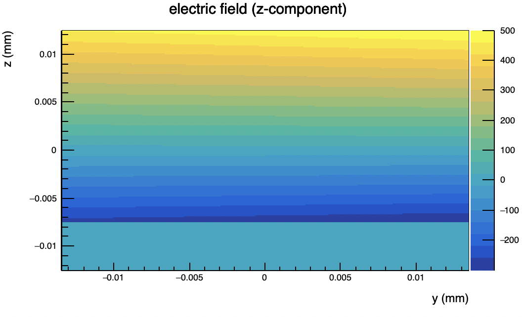
I checked with three different electric field functions and here are the results:

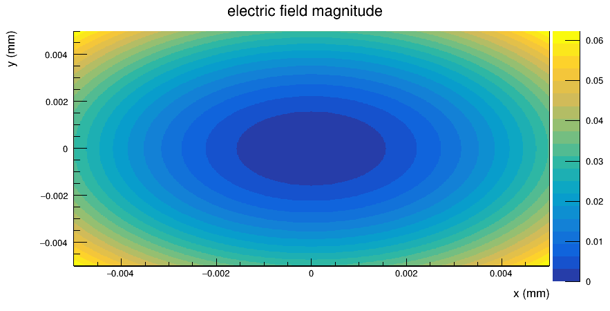
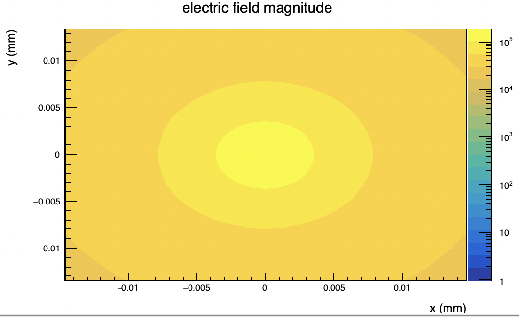
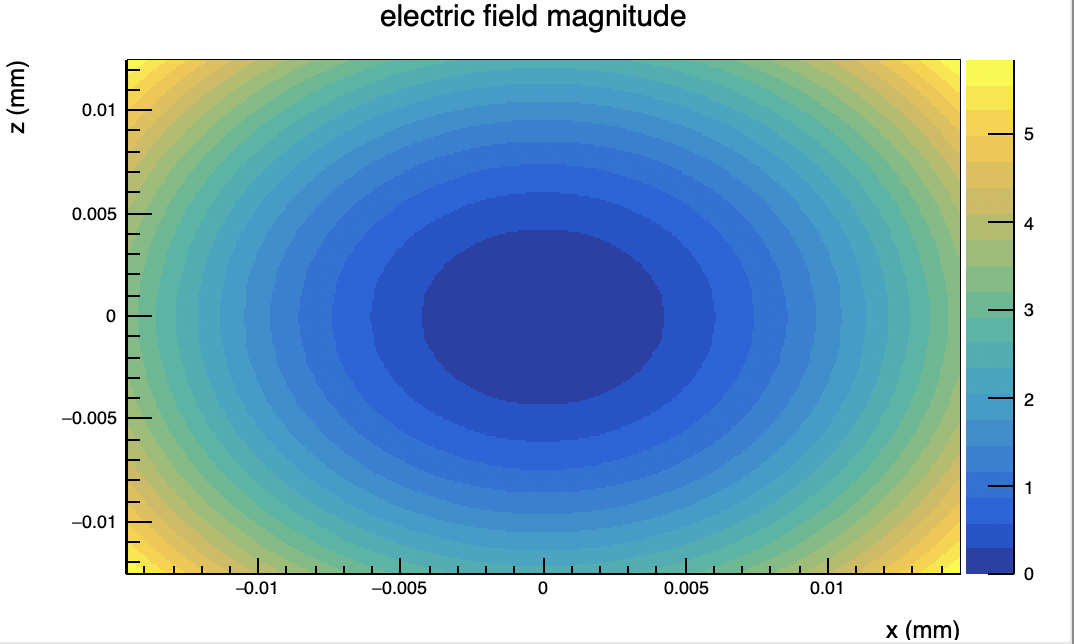
1.	12500V/cm*TMath::Gaus(z,0,1):
ONEDIMENSIONAL::Value of custom field at ( -0.01462,0.01344, -0.0125 ): 12499V/cm
BEFOREPLOT::Value of field_strength  at  (-0.0145908,-0.0134131,0) : 12500V/cm
BEFOREPLOT::Value of field_z_strength  at  (-0.0145908,-0.0134131,0) : 12500V/cm
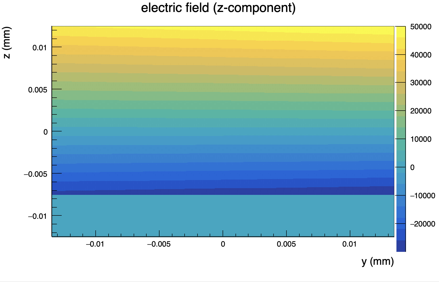
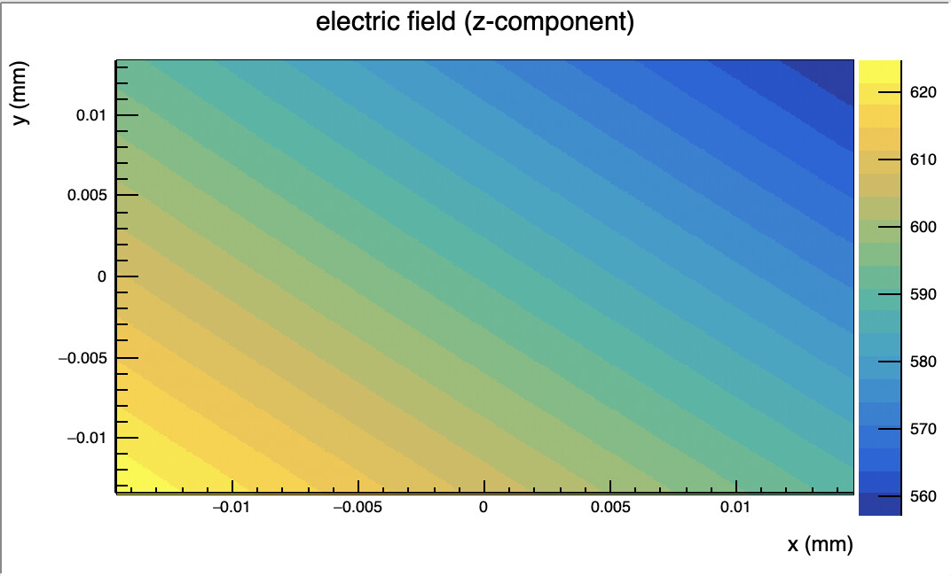
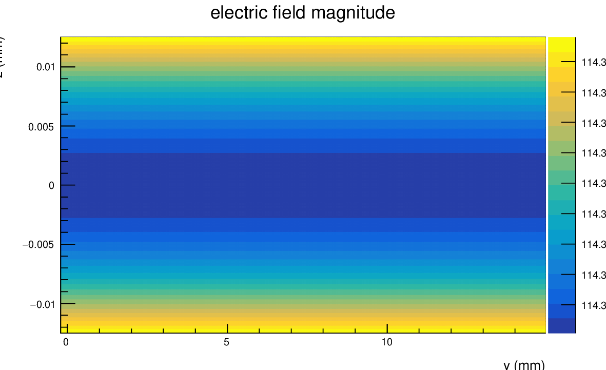
2.	12500V/cm*TMath::Gaus(y,0,1):
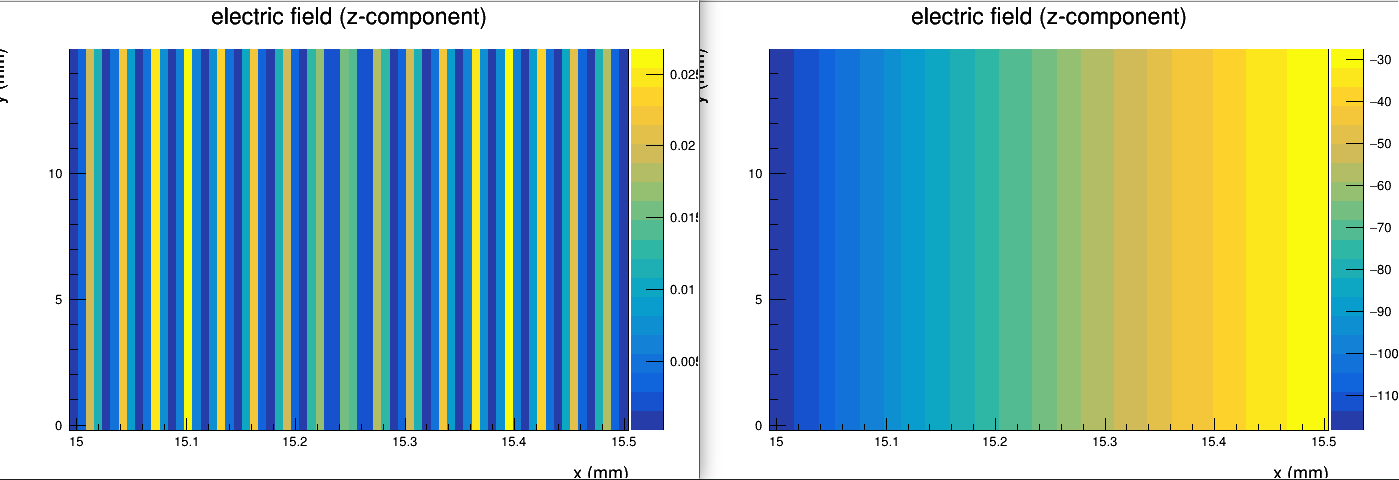
ONEDIMENSIONAL::Value of custom field at ( -0.01462,-0.01344, -0.0125 ): 12498.9V/cm
BEFOREPLOT::Value of field_strength  at  (-0.0145908,-0.0134131,0) : 11031.4V/cm
BEFOREPLOT::Value of field_z_strength  at  (-0.0145908,-0.0134131,0) : 11031.4V/cm
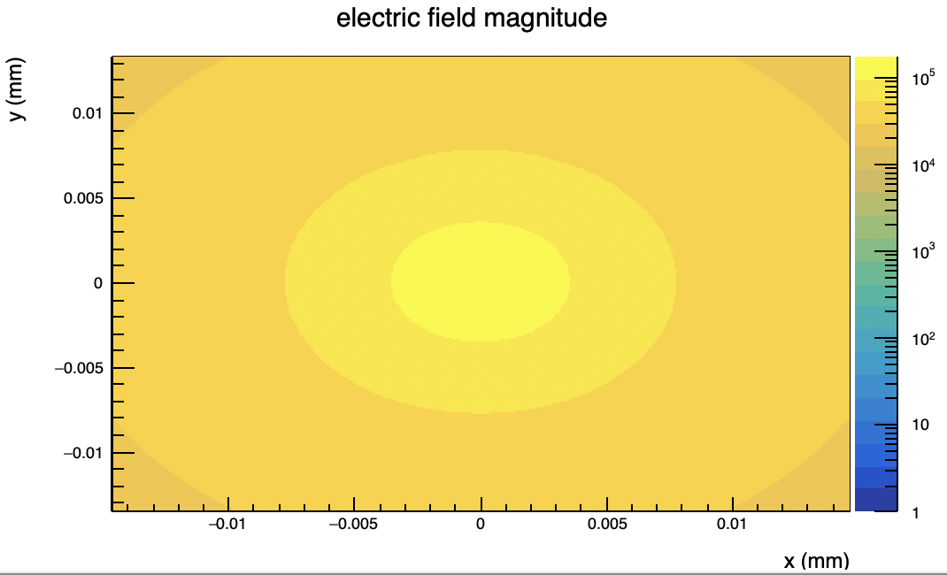
3.	12500V/cm*TMath::Gaus(x,0,1):
ONEDIMENSIONAL::Value of custom field at  ( -0.01462,-0.01344, -0.0125 ): 12498.7V/cm
BEFOREPLOT::Value of field_strength  at  (-0.0145908,-0.0134131,0) : 11031.4V/cm
BEFOREPLOT::Value of field_z_strength  at  (-0.0145908,-0.0134131,0) : 11031.4V/cm

I checked the electric field values using a separate TF3 code. I see that for all three cases the custom electric field is read correctly (in ONEDIMENSIONAL results). But apart from the

TMath::Gaus(z,0,1)

case, for other two equations, the electric field is not plotted correctly. I think that this behaviour is not expected. Can you help me how this function:

void ElectricFieldReaderModule::create_output_plots()
[src/modules/ElectricFieldReader/ElectricFieldReaderModule.cpp · master · Allpix Squared / Allpix Squared · GitLab]

and this function:

FieldFunction<ROOT::Math::XYZVector> ElectricFieldReaderModule::get_custom_field_function(std::pair<double, double> thickness_domain)
[src/modules/ElectricFieldReader/ElectricFieldReaderModule.cpp · master · Allpix Squared / Allpix Squared · GitLab]

talk to each other?
I see this line which sets the electric field:

detector_->setElectricFieldFunction(
get_custom_field_function(thickness_domain), thickness_domain, FieldType::CUSTOM);
[src/modules/ElectricFieldReader/ElectricFieldReaderModule.cpp · master · Allpix Squared / Allpix Squared · GitLab]

and this line which gets the electric field

auto field = detector_->getElectricField(ROOT::Math::XYZPoint(x, y, z));
[src/modules/ElectricFieldReader/ElectricFieldReaderModule.cpp · master · Allpix Squared / Allpix Squared · GitLab]

but could not figure out what is going on between them. Pardon my limited expertise in c++.

Many Thanks,
Arka

[simonspa]

Hi @asantra

cool that you were investigating yourself already, let me try to explain the connection between the functions you were mentioning:

There are three classes involved:

• Detector: this class represents a specific detector placed in your geometry with all the information required for the simulation. This (among others) comprises the following two classes:
• DetectorModel: the detector model describes a detector in terms of its geometry (number of pixels, pitch, sensor thickness etc)
• DetectorField: a detector field is e.g. an electric field (but also e.g. a doping profile) that is attached to a specific detector.

This means, that if you call detector_->setElectricFieldFunction() you take whatever defines your electric field, and store it as that detector’s DetectorField for the electric field. Whenever in the simulation you then ask detector_->getElectricField(...) it will return the electric field from the position given from the DetectorField. The relevant code can be found in the Detector class for storing and for reading.

In the ElectricFieldReader module, what we do is we define a lambda (works similarly to Python, if you know lambdas there) that always returns the electric field, and we pass this lambda to the DetectorField to store and use it. That’s what the function get_custom_field_function() does - it generates a lambda for storage.

Finally, the create_output_plots() method basically only iterates over a single (or multiple) pixel cell and requests the electric field at each of the positions via detector_->getElectricField() - so this function is completely independent of the type of electric field, it only asks the detector about it.

/Simon

[asantra]

Hi @simonspa ,
Many thanks for the clear explanation. Now I start seeing the underline structure of the detector and its field.

I was wondering if what I find

(that the electric field is read fine in
FieldFunction<ROOT::Math::XYZVector> ElectricFieldReaderModule::get_custom_field_function(std::pair<double, double> thickness_domain)

but not in

void ElectricFieldReaderModule::create_output_plots()
)
needs more investigation or this is expected and I need to look for a bug in someplace else. It seems both the functions use local coordinates in a pixel: so it is possible that I am looking at same local position, but in different pixels in different functions. How do I convert the pixel local coordinates into the global coordinate?

Best,
Arka

[simonspa]

Hi @asantra,

your assumption is not completely correct here:

Calling the function returned by get_custom_field_function() directly e.g. with the position (0,0,0) means you are calling your field with an in-pixel position of (0,0,0), i.e. at the center of that pixel. However, detector->getElectricField(...) expects a position in local coordinates of the sensor which is different from the in-pixel coordinates, hence calling it with (0,0,0) you would expect something different. The transformation local coordinates → in-pixel coordinates is performed for you by the DetectorField class in its get() function (if you want to check it out, it’s here).

Cheers,
Simon

[asantra]

Hi @simonspa ,
I noticed that there is an offset in x and y coordinates for the custom ElectricFieldReader. For example, when I used this field function (simple circle in x and y) with alpide chip:

field_function = "[0]*(x*x+y*y)"
field_parameters = 12500V/cm/cm

the electric field in Z that I get is circular in the pixel dimension, but not centred around (0,0) as expected.

But when I do a simple transformation of x and y and rewrite the equation:

field_function = "[0]*((x+0.48538)*(x+0.48538)+(y+0.48644)*(y+0.48644))"
field_parameters = 12500V/cm/cm

then the electric field is circular in pixel dimension and also centered around (0,0) as expected.

I studied the transformation of local coordinates → * in-pixel coordinates*, but could not figure out why the offset is (+0.48538) for x and (+0.48644) in y for alpide chips. Any hint is much appreciated.

Thank you very much,
Arka

[simonspa]

Hi @asantra

thanks for your investigations, you actually tipped me off on where to find the issue. For meshes loaded from TCAD simulations we allow to set an offset and a scale parameter. Now, the scale parameter unfortunately was wrongly initialized leading to a wrong calculation of the lookup position within the pixel when used with something else than a 1d field along z or a mesh field.

I have corrected this now and with your configuration

[ElectricFieldReader]
model = "custom"
field_function = "[0]*(x*x+y*y)"
field_parameters = 12500V/cm/cm
output_plots = true
output_plots_project = z

I get the circular shape without any shifts or other tweak:

(never mind the axes, I think the model I used had a different pitch of 10x10 um)

The code is here: DetectorField: Provide Scale Factors as Fractions of Pixel Pitch (!510) · Merge requests · Allpix Squared / Allpix Squared . It will probably take a few days until this gets reviewed, and some more until we release a patch. But if you are familiar with git and with compiling Allpix Squared, it would be great if you could test this directly.

Please let me know if this now also solves the issues you have seen with your more complex field configurations, and also let me know if you need assistance in testing the patch.

Best regards,
Simon

[asantra]

Hi @simonspa,
Many thanks for looking into this. I have tested the new MR and now I get the circular field without any transformation of x and y. This solves our more complex field configuration as well.
Best,
Arka

[pschutze]

Hi @asantra ,

the MR was reviewed and the code is now also available in the branches master and v2.0-stable, as well in the new tagged version v2.0.1, just in case you’d like to stay on official branches/tags instead of outdated MR branches

Thanks again for reporting this!

Cheers
Paul

[asantra]

Hi @pschutze,
Many thanks for updating the branches. Now I see that with tag 2.0.1, I do not need to transform x and y.

However, I see another problem with the new version: I see that the cluster size plots are significantly different in tag 2.0.1 compared to tag 2.0.0. For example, this is one custom electric field and cluster size plot for tag 2.0.0 with 10k events (since this was buggy, so we transformed x->(x+0.48538) and y->(y+0.48644)).

When I used the same custom electric field (and 10k events) for tag 2.0.1 (and no transformation of x and y), the cluster size plot is very different.

We looked at the cluster charge plot for v2.0.1

and v2.0.0

and do not see any significant change. Is there any change in the clustering algorithm for tag 2.0.0 and tag 2.0.1? I could not find this from the git compare. Please let me know if you need more information from me.

Thanks again,
Arka

[pschutze]

Hi @asantra ,

I’ve been trying to reproduce your results, but I get different results. Would you mind posting your current configuration for retrieving the above plots?

Thanks and cheers
Paul

[asantra]

Hi @pschutze,

Right now, we cannot make the electric field that we are working with public. I tested with a simple electric field function. Even with that we see consistently low cluster size in 2.0.1. Here is the configuration file:

[Allpix]
number_of_events = 1000
log_level = "WARNING"
detectors_file = "tutorial-geometry.conf"
experimental_multithreading = true
root_file = "modules_customElectricFieldLOCAL.root"

[GeometryBuilderGeant4]


[DepositionGeant4]
physics_list = "FTFP_BERT_EMY"
enable_pai = true
particle_type = "Pi+"
source_type = "beam"
source_energy = 120GeV
source_position = 0um 0um -200um
beam_size = 0.5mm
beam_direction = 0 0 1
number_of_particles = 1
max_step_length = 1.0um





[ElectricFieldReader]
model = "custom"
log_level = "WARNING"




######################################
##### simple field ###################
######################################


field_function = "[0]*(x*x+z*z)"
field_parameters = 12500V/cm



################################################
#### other electric field reader parameters ####
################################################



#### other parameters in electric field #####
depletion_depth = 25um
output_plots = 1




[GenericPropagation]
temperature = 293K
charge_per_step = 5
timestep_min = 0.5ps
timestep_max = 0.5ns
integration_time = 20ns
output_plots = 1


[SimpleTransfer]
output_plots = 1


[DefaultDigitizer]
log_level = "WARNING"
electronics_noise  = 10e
threshold          = 120e
threshold_smearing = 5e
output_plots = 1


[DetectorHistogrammer]
log_level = "WARNING"
output_plots = 1

[ROOTObjectWriter]

This is the tutorial geometry config:

[Stave00]
type = "alpide"
position = 0mm 0mm 10mm
orientation = 0 0 0

For tag 2.0.0, we transformed x->(x+0.48538) and y->(y+0.48644) in the electric field equation. We used the CVMFS built versions, so

tag 2.0.0: source /cvmfs/clicdp.cern.ch/software/allpix-squared/2.0.0/x86_64-centos7-gcc10-opt/setup.sh

and

tag 2.0.1: source /cvmfs/clicdp.cern.ch/software/allpix-squared/2.0.1/x86_64-centos7-gcc10-opt/setup.sh

Best,
Arka

[pschutze]

Dear @asantra ,

can you confirm that you are using the correct units for the fields you were comparing? The example you sent me does not, that’s why I’m asking:

field_function = "[0]*(x*x+z*z)"
field_parameters = 12500V/cm

as x is in units of length, this will be field = voltage x length x length x length = voltage x length, which is incorrect. With the changed coordinate transformation this could make a difference.

I tried with a couple of fields with correct units and I get similar cluster size distributions.

In addition: Did you check that the electric field is the same for both configurations not only at the x-y cut you are showing but also at different positions?

Cheers
Paul

[asantra]

Hi @pschutze,
I fixed the problem of units in the config file. Now the config file is this one:

[Allpix]
number_of_events = 100
log_level = "WARNING"
detectors_file = "tutorial-geometry.conf"
model_paths = "/storage/agrp/arkas/AllPixGrid/Threshold"
random_seed_core = 1234
root_file = "modules_customEelectricField.root" 

[GeometryBuilderGeant4]

[DepositionGeant4]
physics_list = "FTFP_BERT_EMY"
enable_pai = true
particle_type = "Pi+"
source_type = "beam"
source_energy = 120GeV
source_position = 0um 0um -200um
beam_size = 0.5mm
beam_direction = 0 0 1
number_of_particles = 1
max_step_length = 1.0um







##### for customized electric field


################################################
#### custom electric field prepared by Noam ####
################################################


[ElectricFieldReader]
model = "custom"
log_level = "WARNING"


######################################
########## simpleField #########

field_function = "[0]*((x)*(x)+(z)*(z))"
field_parameters = 12500V/cm/cm/cm


###### other electric field parameter #### 


depletion_depth = 25um
output_plots = 1
output_plots_project = y








[GenericPropagation]
temperature = 293K
charge_per_step = 5
timestep_min = 0.5ps
timestep_max = 0.5ns
diffuse_deposit = true
integration_time = 20ns

[SimpleTransfer]


[DefaultDigitizer]
electronics_noise  = 10e
threshold          = 120e
threshold_smearing = 5e
#output_plots = 1


[DetectorHistogrammer]
output_plots = 1

[ROOTObjectWriter]

I ran ~20k events for each of the allpix tags.
These are the electric field and cluster size for allpix tag 2.0.1

These are the electric field and cluster size for allpix tag 2.0.0

The cluster size shapes that I get for the two versions are different.

How do I draw the electric field distributions at different positions? This can be a good cross-check that indeed I apply the same fields in two versions. I naively use

output_plots_project = y

to give me x-z distribution (at y=0) of the electric field.

Best,
Arka

[asantra]

Hi @pschutze ,
We have another query related to how the Allpix understands the unit in a custom electric field. Since Allpix uses TF3 in the back, we think for the following case:

field_function = [0]*exp(-x/3.13)
field_parameter = 12500V/cm

the argument inside the exp is just the numbers and unitless. Therefore, the overall unit to the field is coming from the parameter [0].

We are thinking of another possibility:

field_function = [0]*exp(-x/[1])
field_parameter = 12500V/cm, 3.13cm

where the x inside exp has the unit of length and we divide by another length unit to make the argument inside the exp dimensionless.

Which way should we go? We want to understand if Allpix expects and actually checks that all arguments inside math functions are dimensionless.

Thank you once again,
Arka

[pschutze]

Hi @asantra ,

first, you can change the way you plot fields with excatly this (and some more) parameters. From the Readme:

• output_plots_project : Axis to project the 3D electric field on to create the 2D histogram. Either x, y or z. Only used if output_plots is enabled.
• output_plots_projection_percentage : Percentage on the projection axis to plot the electric field profile. For example if output_plots_project is x and this parameter is set to 0.5, the profile is plotted in the Y,Z-plane at the X-coordinate in the middle of the sensor. Default is 0.5.
• output_plots_single_pixel: Determines if the whole sensor has to be plotted or only a single pixel. Defaults to true (plotting a single pixel).

For your case, I agree I find matching fields looking at different projections. However, when I do output_plots_single_pixel=false (which plots the field over the full sensor) I see the following, e.g. for

[ElectricFieldReader]
model = "custom"

field_function = "-[0]*((x+0.48538)*(x+0.48538)+z*z)" # for v2.0.1: field_function = "[0]*((x)*(x)+(z)*(z))"
field_parameters = 12500V/cm/cm/cm

depletion_depth = 25um
output_plots = 1
output_plots_project = x
output_plots_single_pixel = false

v2.0.0:

v2.0.1

As the application of local fields to global fields were changed from v2.0.0 to v2.0.1, the transformation you did in v2.0.0 does not seem to be enough to get the correct field throughout the full sensor.

Additionally I compared the fields in the x plane and you can see that the pattern that should repeat for every pixel is present in v2.0.1 (left) but not in v2.0.0 (right):

As the field is just very different in both cases (and much stronger in large regions for the old version), the cluster size changes as well. With the plot above in mind: does anything speak against continuing with v2.0.1 or was this just a cross-check? Thanks again for spotting this issue!

Also, please let me know if there are further issues with this.