Dear Allpix-Squared experts,
Hello 
We are currently performing simulation studies of irradiated 100 um thick, 50x50 um2, n-in-p planar sensors. The simulations involve 120 GeV pions injected at the center of the pixel matrix (10mm, 4.8mm) at an eta value of 0 and a 2T magnetic field oriented along Y. To compensate for Lorentz angle deflection, our detector is tilted around Y by -0.25Rad.
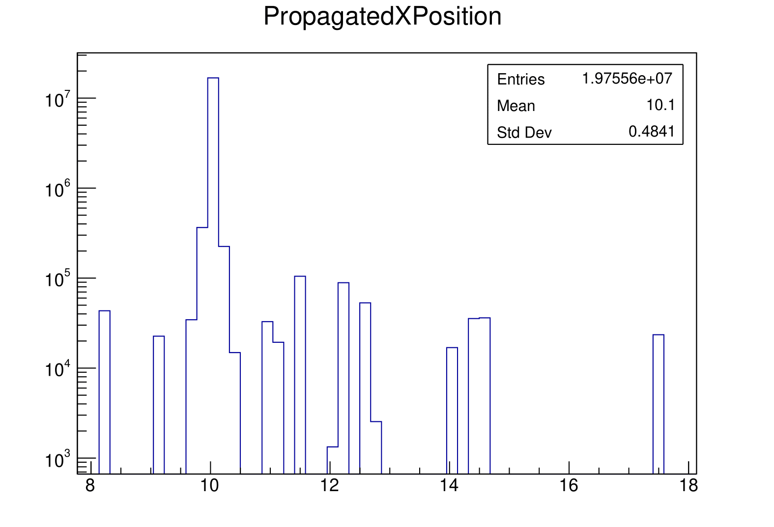
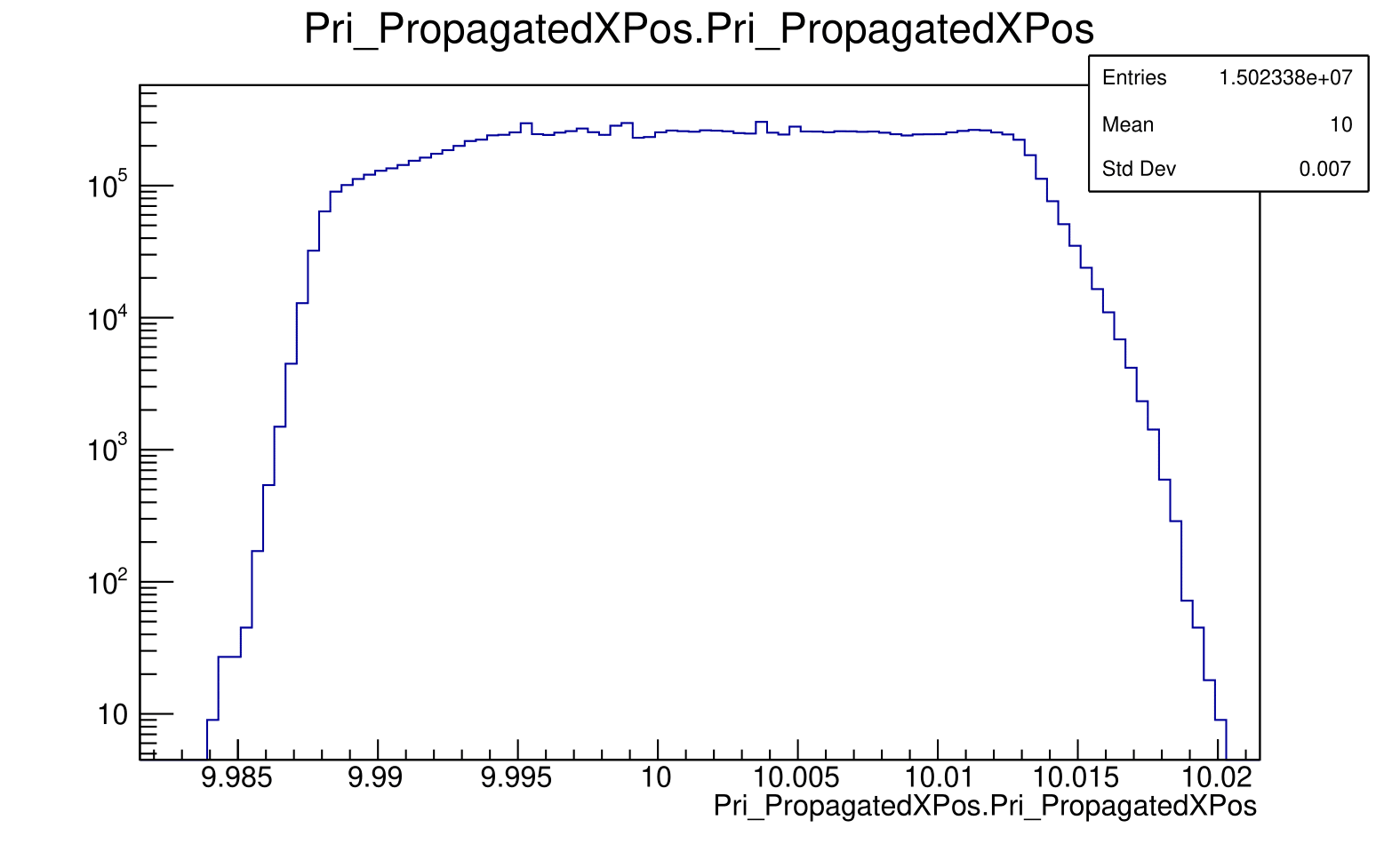
In our studies, we’ve produced the distribution of the PropagatedXPosition of the charge carriers using a macro attached below. As you can see in the attached figure, we see a somewhat discontinuous distribution with spikes (X axis is in mm).
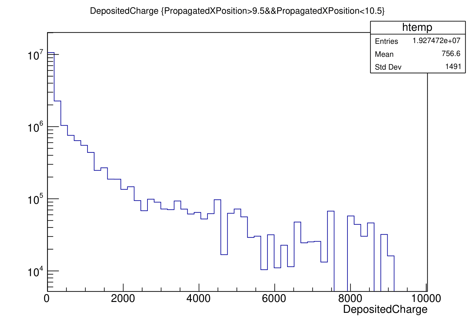
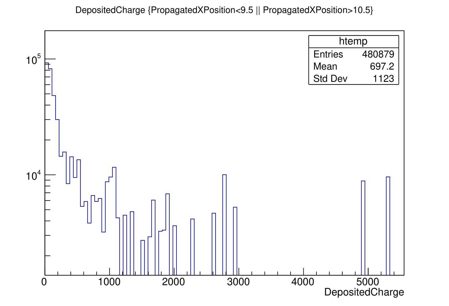
Initially, we hypothesized that the spikes at large PropagatedXPositions (17.5mm) might corresponded to delta electrons. To validate this hypothesis, we examined the distribution of deposited charges at different PropagatedXPosition regions as you see in the plots attached below. Surprisingly, both distributions showed a mean charge of approximately ~700e electrons, leading us to dismiss our initial delta electron hypothesis.
We are reaching out to seek your help to understand peaks observed at large values of PropagatedXPositions. Any insights or guidance you can provide would be greatly appreciated.
Thanks a lot!
@mbomben and Keerthi
Relavant files:
- Main config: CERNBox
- Detector Config: CERNBox
- Macro for PropagatedXPosition: CERNBox
- Electric field map: CERNBox
5)Weighting field map: CERNBox
Ok, let’s be more verbose…
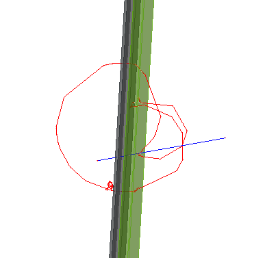
I followed these spikes and they origin from secondary particles - and as you’re operating in a magnetic field, they keep coming back.
For you to follow up on these:
To hunt those down, I ran your macro with customized printouts to see which events are affected and then just ran one of those events. You can do so e.g. by setting these options:
skip_events = 72
number_of_events = 1
In this particular event I find, besides the initial pion, a secondary particle that deposits charges, and I’m doing this …
    auto mcp = prop_charge->getMCParticle();
    auto mct = mcp->getTrack();

    std::cout << "Charge " << prop_charge->getCharge() << " at x=" << propagated_x_pos << " ParticleID: " << mct->getParticleID() << " Process: " << mct->getCreationProcessName() << " Ekin_ini: " << mct->getKineticEnergyInitial() << std::endl;
to get more info, and one of the output lines reads
Charge 0 at x=15.447 ParticleID: 11 Process: hIoni Ekin_ini: 1.66844
. Hence we’re dealing with an electron created in an ionisation process with an initial kinetic energy of 1.67 MeV. Now, if you’d like to ignore these particles in your data postprocessing, you can of course just filter on the above properties.
I hope this is of help. The track in the post before looks quite nice, though!
Cheers
Paul
One additional bit of information:
the term MCParticle in APSQ refers to any particle within a sensor. A looping particle that enters the sensor multiple times might create multiple separate (primary) MCParticles.
Use the MCTrack objects to link them together!
Simon
Hello @pschutze and @simonspa,
Happy new year! 
I just wanted to share a quick update and get your thoughts on the study of the spikes seen in PropX distributions.
I’ve been diving into the simulation details, and with your detailed guidance, I’ve filtered out MC particles based on their initial kinetic energy and primary MC particle status in my analysis macro. Here are the three cases I’ve seen (in brackets how I filter them in my code):
-
Events with only primary pions (mcp->isPrimary() && Ekin_mct == 120000)
-
Events with secondaries re-entering the sensor, aka “fake” primaries (mcp->isPrimary() && Ekin_mct != 120000)
-
Events with secondaries passing through the sensor without re-entering aka “actual” secondaries (!mcp->isPrimary())
Out of 1000 events with 120 GeV pions, 93 had secondary emissions. Among those, 73 had secondary electrons passing through the sensor, and 20 had secondary electrons re-entering as new “fake” primaries.
The left plot shows the distribution of PropagatedXPositions of primaries only, the right one corresponds to the PropX distribution of secondaries re-entering the sensor and the bottom left corresponds to the secondaries passing through the sensor.
As you can see after filtering the secondaries out, the PropX distribution is continuous, very narrow and centred around 10mm
The analysis macro is attached here. It’d be great if you could kindly let us know if you see any fallacies in this approach.
Thank you so much,
@mbomben and Keerthi
Hi @knakkali ,
I’m glad to see that these hints were helpful. I did not read/try/test the code in full length, but I have a few comments:
- In line 143 and 156 you check for the energy. Be careful here, as
Ekin_mct is a double, this comparison (Ekin_mct==120000) might not be stable. Better practice would be to calculate the difference and check whether this is a low number (e.g. compare with epsilon)
- You could even get rid of the comparison above using more features of the
MCTrack object. There’s e.g. the method int getCreationProcessType() or std::string getCreationProcessName() which you could use. You can identify real primary particles via their creation process, which would be -1 or none for the methods above.
Cheers
Paul
Hi @pschutze and @simonspa ,
We wanted to update you guys on our study. Now that we’ve understood the origin of spikes in the PropXPosition distributions, we have incorporated a filter for secondary particles in our analysis macro. Consequently, we see a very smooth and continuous distribution of PropXPosition, as illustrated in my previous post. Additionally, we have a comparison of the PropX distribution with our closure test, using the [LUTPropagator] module we are developing. Enclosed below are the results, showing excellent agreement in both mean and FWHM of the distributions.
Continuing with our strategy of filtering secondary particles in the analysis script, we had a look at the distribution of PixelMaximumCharge per event and compared it with our closure test, as shown below. The relative error in mean between APSQ full simulation and our closure test is 5.7%, while the error on sigma is as high as 44%, as you see below.
We also examined these plots without filtering for the secondaries, and we see an excellent agreement in both mean and standard deviation, as depicted below.
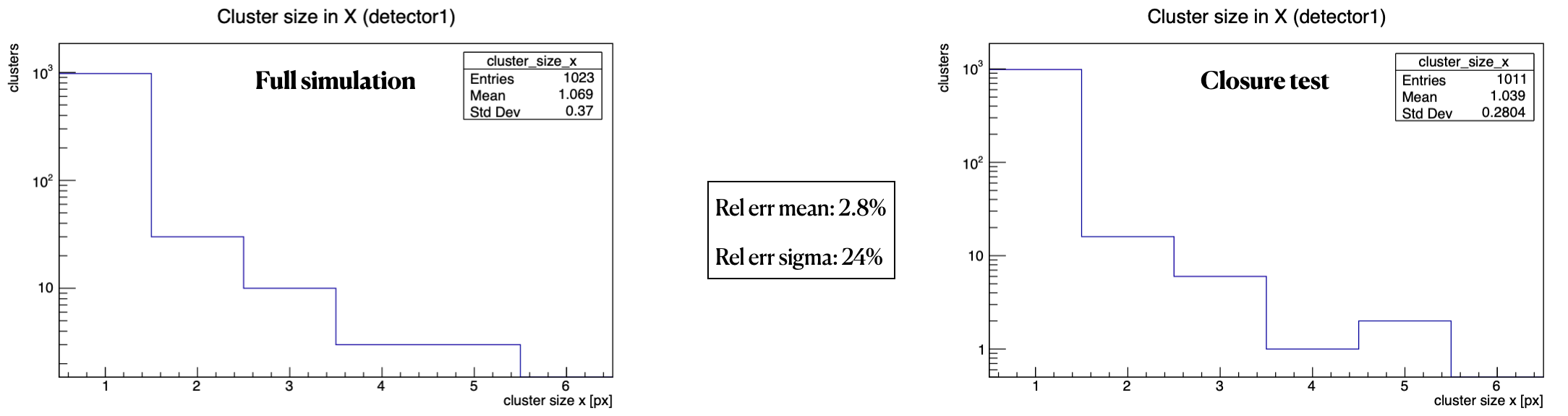
The cluster size in x and the cluster charge variables from the [DetectorHistogrammer] module, which (I think) includes the secondaries, also exhibit excellent agreement, as you see in the plots below.
We are currently trying to finalise our analysis strategy, specifically regarding whether to filter the secondaries in APSQ full simulation and taking a step back and looking at all the plots together makes me wonder whether the differences observed in PropX with secondaries are intrinsic to this distribution coz all other plots, including those involving secondaries, demonstrate a rather good closure, and we wanted to get your opinion on this matter.
Thanks a lot,
Marco and Keerthi
Dear @knakkali ,
to understand these results in greater detail, could you please explain what the “Closure Test” is and what the differences between the graphs are?
Thanks and cheers
Paul
Hi @pschutze ,
Oh!!I’m terribly sorry. I should’ve put the context in a better way. We are working on developing a lightweight algorithm to model radiation damage effects in MC events within the ATLAS detector for HL-LHC based on charge re-weighting from look-up tables (LUTs), and we are utilizing ALPSQ for generating these LUTs. We have obtained estimates for the charge collection efficiency, average Lorentz angle, and average free path of carriers as functions of charge deposition depth (z).
Having successfully generated our LUTs using APSQ, our next step involves validating this new strategy through a closure test and the strategy we used is as follows:
- Simulate charge deposition
- Determine final position and fraction of induced charge using our lookup tables
- Proceed with transfer and digitization steps
- Compare the results at step 3. with the ones obtained using the full APSQ simulation chain
For step 2, we have developed a new module ([LUTPropagator]) that takes in our three LUTs and calculates the fraction of induced charges and the final position of charge carriers.
The plots labeled as “Closure test” represent the results obtained using our [LUTPropagator], while those labeled “Full simulation” correspond to results obtained using the [TransientPropagation] module in APSQ.
For more info on the studies we’ve done till now, I’ve included a link to a talk we presented at the RD50 meeting in December '23: RD50_talk
Please do let me know if you have further questions or require additional info
Thanks a lot
Keerthi
Hi @knakkali
thanks a lot for the update, the results really look fantastic! I hope you are planning to come to the APSQWS5 to present these!
Any plan for opening a merge request any time soon? 

All the best,
Simon
1 Like
Hi @simonspa ,
I hope you are planning to come to the APSQWS5 to present these!
Yes, we are excited to present the results at the APSQ WS once we finalise the analysis strategy on whether or not to filter out the secondaries. Can I maybe ask your option on this? Do you think this is feature of PropX plots considering we have a rather good closure for all other variables while including the secondaries ?
Any plan for opening a merge request any time soon?
Yeah, Sorry about this. I just keep pushing this down my to-do list as new urgent deadlines pop up on top. I’ll make it a priority to do the code cleanup and make an MR in the next couple of days
Hi @knakkali
Given that you understand where the effect comes from (looping particles) and that this is nothing that will affect your description of the cluster, I would consider this fine.
Does this answer your question? I’m not 100% sure I caught what you wanted to know…
Simon
Hey @simonspa,
Thanks a lot for getting back to me!
So, your input pretty much addresses my question. I’ve been going back and forth on whether to ditch the secondaries in my data post-processing. When I filter them out, I do see some solid closure in the PropX plots, but other plots, like PixelMaxCharge, don’t quite agree as well without the secondaries.
I’m leaning towards your argument that the cluster charge is the key player in reconstruction. The agreement between the closure test and the APSQ full simulation, including the secondaries, is looking quite good. And as you rightly pointed out that the cluster description is unaffected by these looping secondaries, I think I’ll stick with keeping the secondaries in my analysis.
Thanks a lot!
Keerthi