Dear developers,
I am currently working on a simple monolithic detector made of a 3x3 pixel matrix, with pixel pitch of 25 um and thickness of 50 um.
I am simulating 100 events, using the module [DepositionPointCharge], with source_type = “mip”, which traverses the detector in different positions. Moreover, I use the [TransientPropagation] and [PulseTransfer] modules.
I have some questions which I hope can be clarified.
- First of all, I wonder if the WeightingPotential, in case of a pixel matrix, is automatically replicated for every pixel, as it happens for the electric field. (It has been calculated for a single pixel). I specify the use of the parameter induction_matrix = 3, 3 in the propagation module.
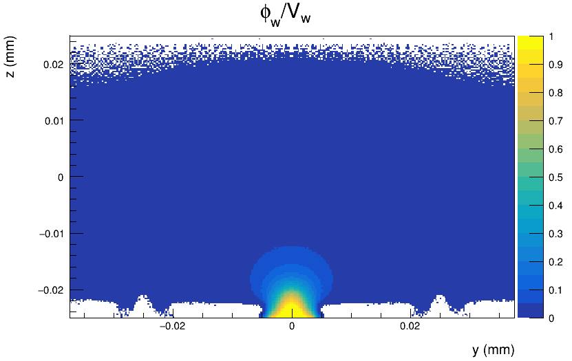
The Weighting Potential maps that I obtain from the [WeightingPotentialReader] module are as the following:
-
With regard to the induction_matrix parameter of the [TransientPropagation] module, I read in the manual that, in case of a larger matrix, a value of 3, 3 should be sufficient and the simulation time remains reasonably small. I wonder, for example, if one has a 5x5 pixel matrix, which 3x3 pixel sub-matrix is considered in the last case.
-
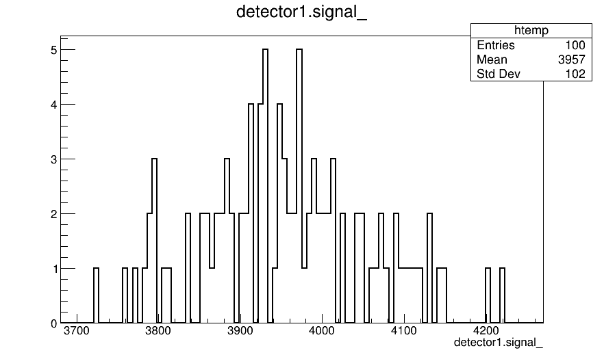
Another very quick question concerns the PixelHit object in the output file of the simulation, from which I pick this detector_signal histogram:
Then, I used the ROOT macro constructComparisonTree.C, supplied by Allpix and, in the file output.root, I also find the total_charge histogram, that I report below
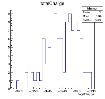
What’s the difference between the two graphs? In particular, why are they different?
-
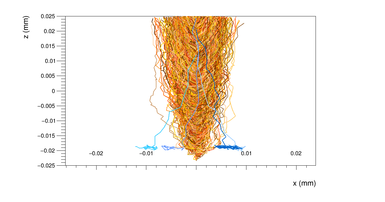
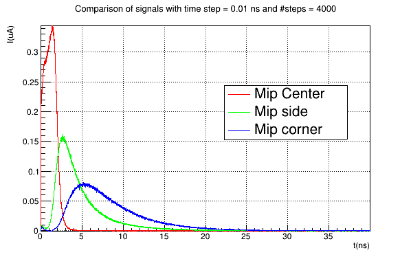
Finally, in the module [PulseTransfer], I don’t enable the collect_from_implant parameter and I obtain signals like this:
Since the [TransientPropagation] module simulates the transport of both electrons and holes, is this signal the result of a sum of the electron and hole signals?
Thank you in advance for your support!
Best regards,
Chiara
Dear @cferrero
let me try to answer your questions one by one.
-
The weighting potential behaves differently than an electric field because it has different boundary conditions. You calculate it by setting your electrode of interest on unit potential an all other electrodes to zero. This means also electrodes of neighboring pixels if you look at a 3x3 matrix. This allows the weighting potential to extend beyond your single pixel cell and the charge carrier can induce (small) currents in neighbor pixels.
Your weighting potential looks like it is occupying only a single pixel cell, so setting an induction matrix of 3x3 pixels will not give you anything - the weighting potential in neighboring pixels with respect to the position of the charge carrier will always be zero, hence no induction of charges. So unless you change your weighting potential to cover a larger volume, you can as well set the induction matrix to 1x1 and save a factor 8 in computing time.
What strikes me in your plot is that your unit potential electrode is on the backside of the sensor, I believe you should invert the z axis of your potential.
-
As hinted already in the previous answer - the “induction matrix” does not refer to the size of your pixel matrix but simply the submatrix of electrodes/pixels around the position of your current charge carrier that we will calculate induced currents for. Let’s say you are observing a charge carrier somewhere in pixel (1,1) then we would – for every step – calculate the induced currents in pixels (0,0), (0,1), (0,2), (1,0), (1,1), (1,2), (2,0), (2,1), (2,2), so a 3x3 matrix around your charge carrier. For this to have any effect, your weighting potential needs to be of that size, i.e. 3x3 pixels wide - otherwise the weighting potential at the position of the charge carrier with respect to any of the neighboring pixels will always be zero.
-
I would have to look closer at which histograms you are looking at. Could you provide me the configuration you are using to write the data? Where do you plot the detector.signal_ histogram from?
-
Yes, this is the total induced current in the electrode, containing the contribution from both electron and hole drift as required by Ramo’s theorem.
I hope this could shed some first light on your questions, feel free to dig deeper, I’m happy to answer!
/Simon
Dear @simonspa,
thank you for the quick reply.
-
So, if I understand correctly, I should have an electrostatic potential defined for a 3x3 matrix, in order to compute the weighting potential for all the pixels in the matrix. In this way the collection electrode of interest (where I read the signal) will have a unit potential, and all others will have a zero potential.
-
Of course, here’s the config. files I’ve used.
Simulation.conf (2.0 KB)
detector.conf (252 Bytes)
I find that histogram in the output file of the simulation, named “output_tcad_field_simulation_iv_50.root” , than I open the PixelHit tree, the detector branch and the signal leaf.
-
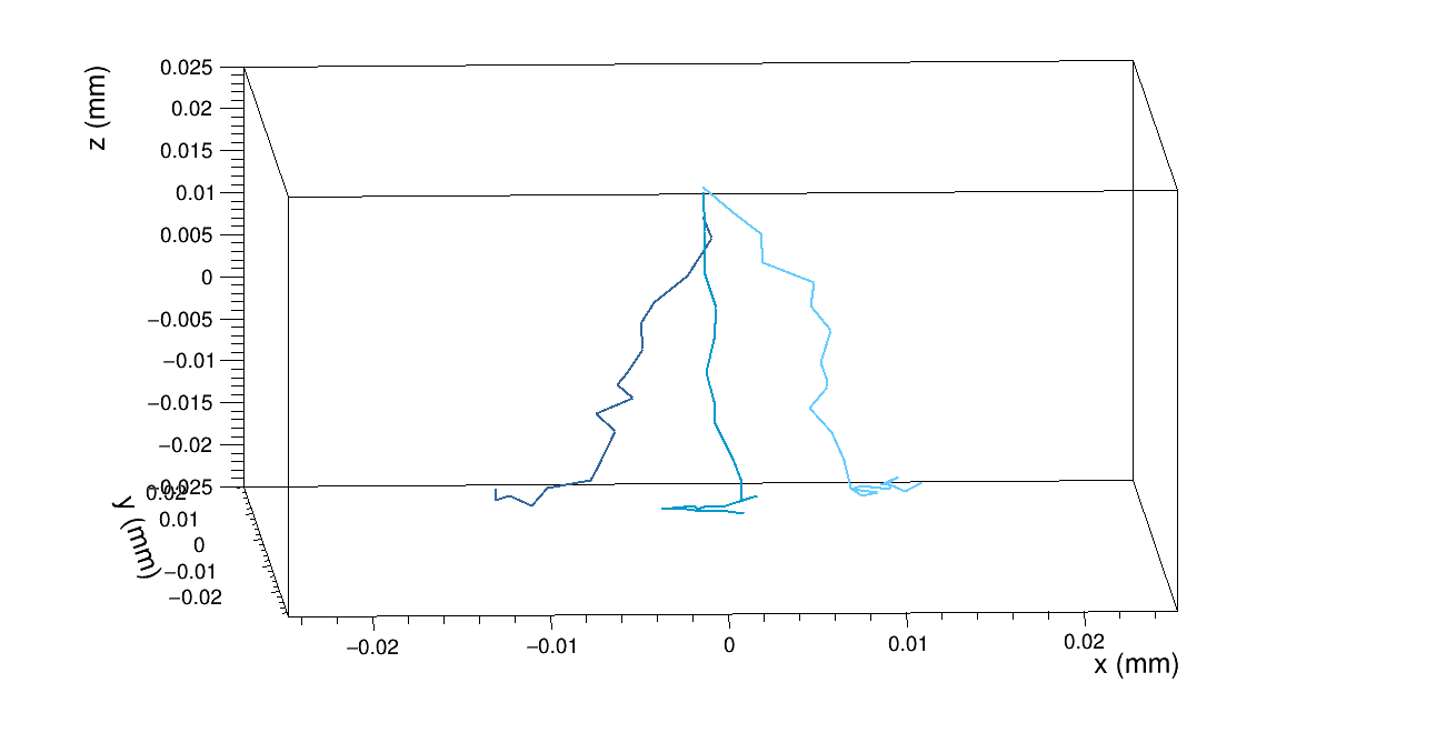
Another doubt I would like to clarify concerns the GenericPropagation module. I tried different configurations for one pixel, with the output_linegraphs parameter setted to true, but the line plots that I obtained confused me.
For example, if set Propagate_electrons to true and propagate_holes to false,
integration time = 25ns,
lines_at_implant = true,
I obtain the following line plot
Than, if I set lines_at_implant = false:
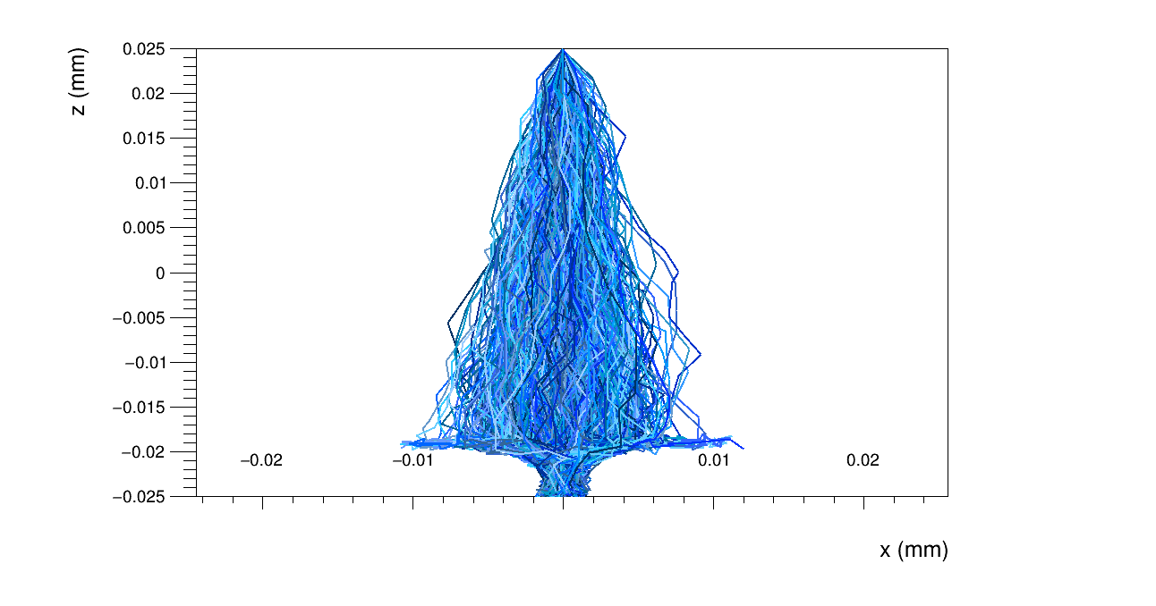
and when I propagate also the holes, with the parameter lines_at_implant = true
I obtain the following line plot:
I wonder why I have so many hole lines, while only a few electron lines.
This is the configuration I’ve used:
[GenericPropagation]
type = “Arcadia_25um”
temperature = 293K
charge_per_step = 1
timestep_min = 1ps
timestep_max = 5ps
timestep_start = 1ps
spacial_precision = 0.1nm
output_plots = true
integration_time = 25ns
propagate_holes = true
propagate_electrons = true
output_linegraphs = true
output_plots_step = 100ps
output_plots_lines_at_implants = true
with the DepositionPointCharge module
[DepositionPointCharge]
log_level = “INFO”
model = “fixed”
number_of_steps = 1000
source_type = “mip”
position = 0um 0um 0um
spot_size = 0.01um
Thanks a lot,
Chiara
Hi @cferrero
let me first answer your last question and then prepare a more elaborate answer for the rest. 
“Implants” here always refers to the readout side of the detector, which by definition of the local coordinate system is a the positive z axis. Looking at your plots this tells me
- currently your electric field is oriented such that electrons drift to the backside and holes to the front side (implant side)
- the reason for the three lines showing up at the top of your sensor is that somehow they started within the implant and might therefore be considered by the selection (this could be a bug, I have to check)
- If your sensor should collect holes I think you have the same issue as with the weighting potential, you need to rotate it around to get the implant up to positive
z.
Does that clear up the confusion a bit?
/Simon
Hi @cferrero
concerning the induction matrix and weighting potential: I made some drawings which I hope help to explain the concept. 
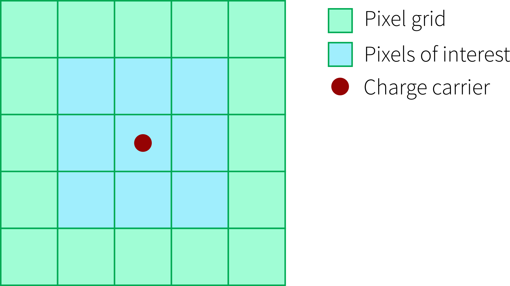
The situation
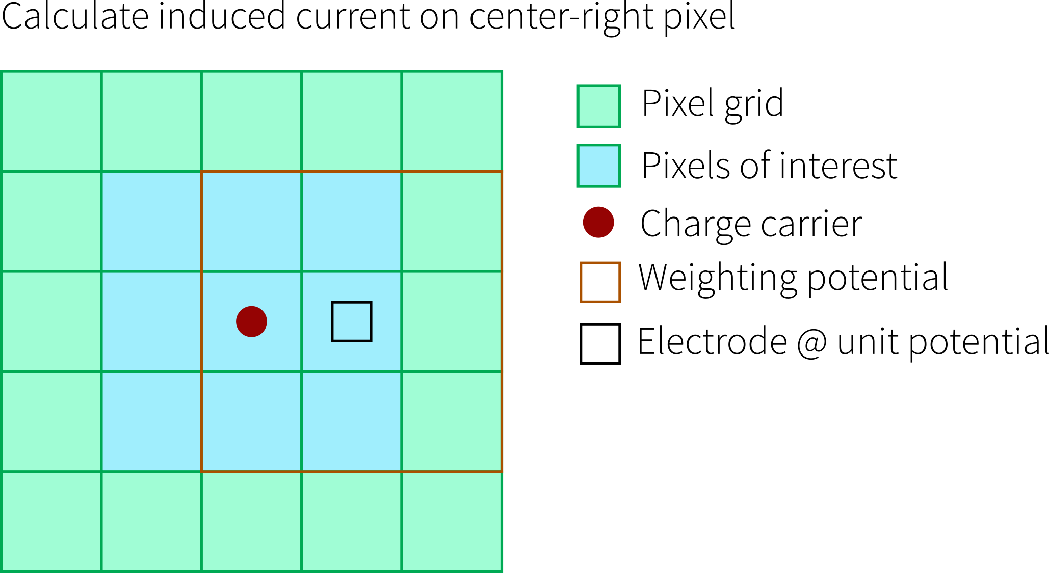
You have a charge carrier located in a pixel, here we look at one charge carrier (red) in the center pixel of a 5x5 pixel sensor (green). We are now interested in how much current this carrier induces in the pixel it is in as well as the surrounding ones, se we define a 3x3 induction matrix (blue):
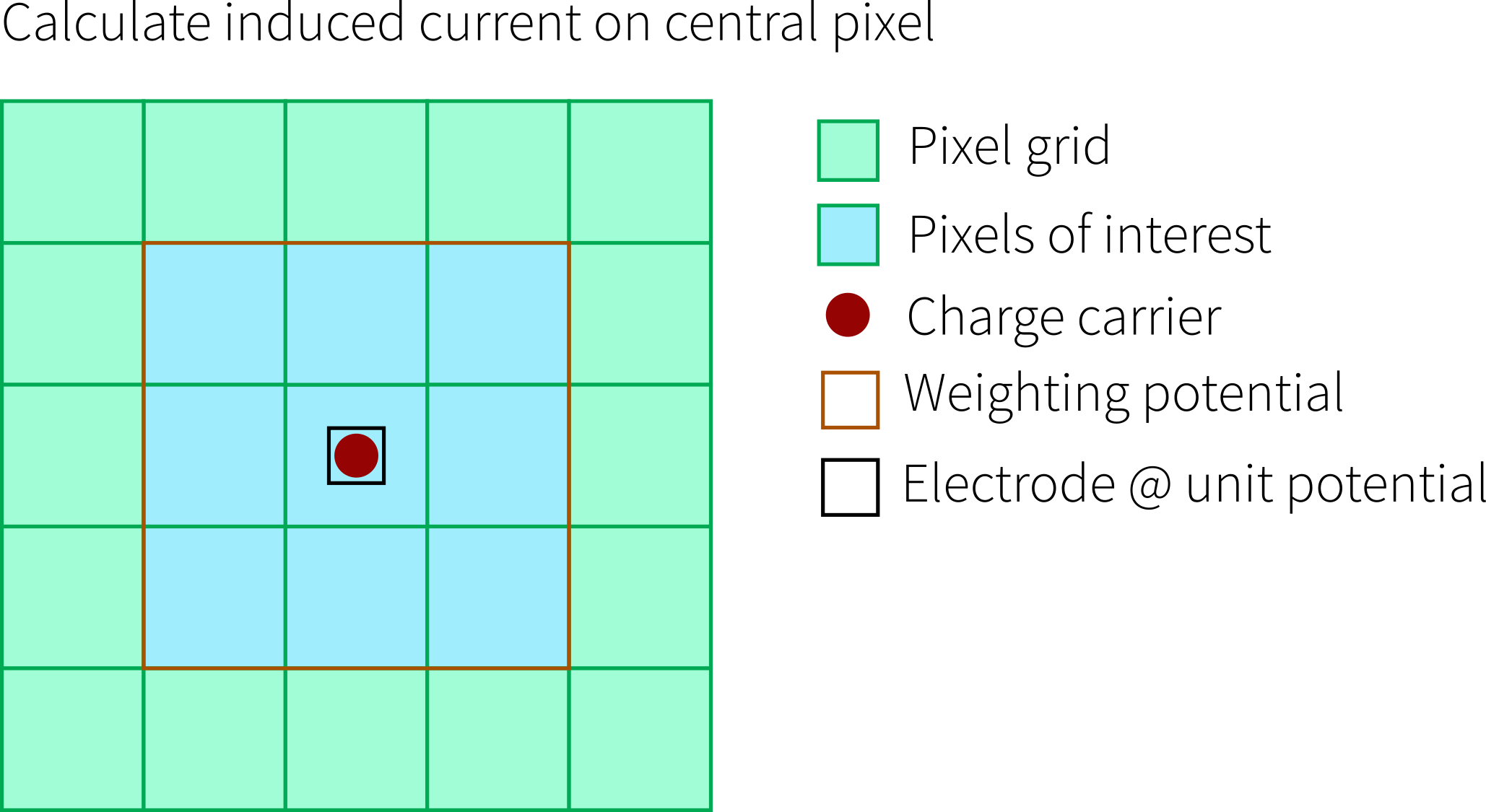
The Weighting Potential
Now we need a weighting potential in order to use the Ramo theorem (orange). The theorem tells us that we can use weighting potential differences to calculated induced currents. Important here is that only one electrode is set to unit potential, all others to ground - and we always calculate the induced current for exactly this electrode. So for the picture below, this would be the central pixel:
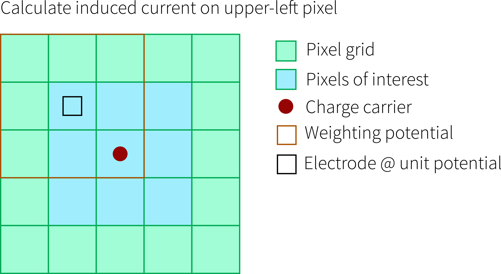
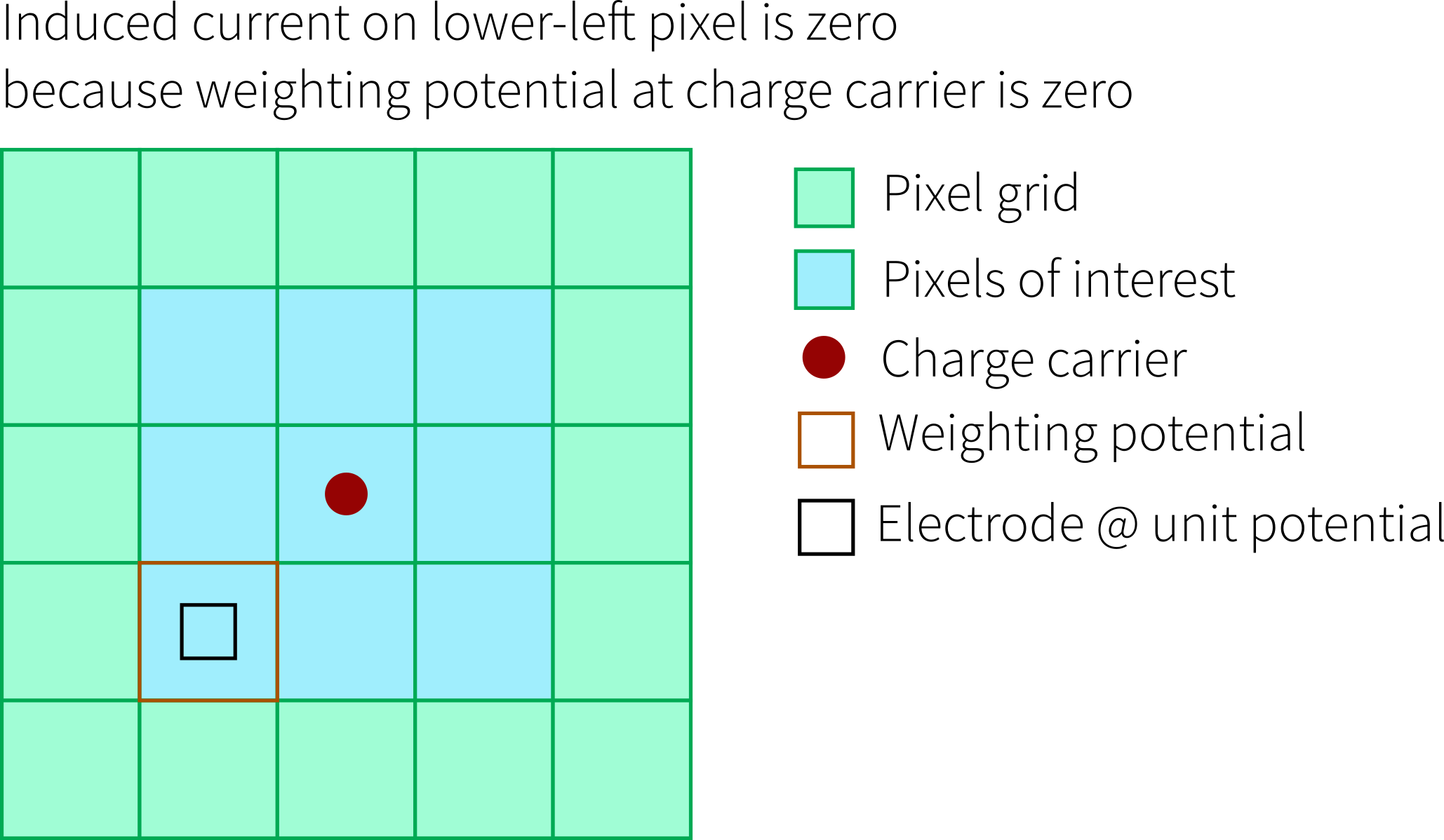
Getting Current for Neighbors
Now it becomes more interesting because we would also like to know the current e.g. in the pixel in the upper left. Therefore we need to shift our weighting potential such, that the unit-potential-electrode is located on that pixel. Then, the charge carriers are somewhere in the lower right of the weighting potential, where it falls off to zero - and we can calculate the (probably small) induced current in that pixel:
This procedure we continue for other pixels:
Conclusion
- if we want the induced current of neighbor pixels, we need to have a weighting potential that is at least as large as the sub-matrix we would like to calculate currents for - because we need to shift the potential around
- if we are only interested in the single pixel the charge carriers are moving below, there is no need for an extended weighting potential and we can use that of a single pixel - we won’t get induced currents in neighbors though, as becomes clear from this drawing:
All the best,
Simon
1 Like
Hi @simonspa
Thank you for your reply!
-
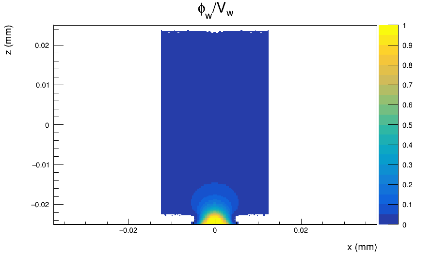
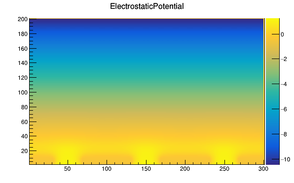
I don’t understand why the readout side of the detector has to be located at the positive z axis. Here’s the electrostatic potential map that I obtain with the Mesh Plotter tool of a 3x3 pixel matrix, where I have 200 divisions on Z and 300 divisions on Y.
My detector should collect electrons.
The collection electrodes are located at small division values in the Z axis and similarly, in the plot of the weighting potential (which now is defined for the entire 3x3 matrix), the collection electrode is located at small Z values (in this case negative z).
Weighting potential for the matrix:
but things look consistent to me. The question that arise to me is: the particle enters the detector from positive or negative z-axis?
-
Thank you for you detailed explanation of how to manage with weighting potentials in the matrix! It has been very useful for me.
So, if I’m interested in reading the current signals from many pixels at the same time, I should put to unit potential all the pixels I’m interested in reading the signals from? Or I can only follow this procedure for one pixel at a time?
Thanks a lot,
Chiara
Hi @simonspa ,
sorry for the delay in the reply. I understand the reason for rotating the z axis and now it works fine!
I am working with @ldecilla on further simualtions and we have a question about the induction_matrix parameter.
We are simulating the incidence of a mip in three different positions over a 5x5 pixel matrix. I have computed a weighting potential map for 1 pixel cell:
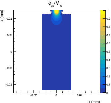
The problem is that if I use the following TransientPropagation’s configuration
[TransientPropagation]
temperature = 300K
charge_per_step = 4
timestep = 0.01ns
integration_time = 40ns
induction_matrix = 3, 3
output_plots = true
I obtain a reasonable charge collection efficiency, like this:
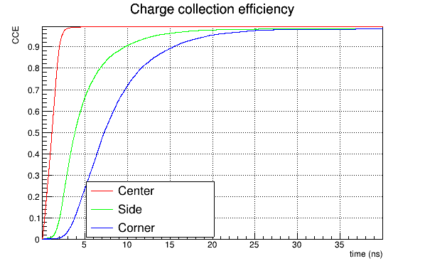
Instead, if I use the induction_matrix parameter setted to 1,1 I obtain:
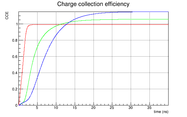
Again, if I use a weighting potential map computed for a 3x3 pixel sub-matrix with the induction_matrix parameter setted to 1,1 , the CCE obtained is reasonable (which seems absurd), while if I use the same weighting potential map but with the induction_matrix = 3,3 I obtain a CCE like the second shown before.
We don’t understand why this happens.
Thank you so much,
Chiara
Hi @cferrero
oh, wow, calling this absurd is an understatement really… Let’s figure out what’s going wrong here, because from your description to me it sounds like you are doing everythong exactly right.
May I ask how you calculate the CCE? I presume you take the induced charge (current over time) divided by the total charge. How do you calculate the latter?
/Simon
Hi @simonspa,
thanks for your reply!
The CCE is calculated as the integral of the current signal (summed over all the pixels → matrix signal) divided by 0.64 fC = 80 eh pairs/um * 50 um (since we are using a mip with DepositionPointCharge.
So actually, what we do not understand is: if I compute a weighting potential map for 1 pixel only, does it make sense to have a 3x3 induction matrix? This leads us to a reasonable collected charge (integral of the current signals from all the pixels together → matrix signal), but it seems to us that we should have a 1x1 induction matrix (as we have a map for 1 pixel only). However, this results in a higher collected charge (integral of the current signal over all the pixels summed together) if the particle (or mip) impacts at the side or at the corner of the pixel.
Does the first case (1x1 weighting potential map and 3x3 induction matrix) scale (“stretch”) the weighting potential map over a 3x3 matrix (so making it unphysical)? Or does it work differently?
On the the way around, if we have a weighting potential map calculated for a 3x3 matrix (with only the central pixel at unit potential), it would seem to us that we have to use a 3x3 induction matrix. But this again results in CCE > 1 for side and corner positions. If we instead fix the induction matrix to 1x1 with a 3x3 weighting potential map, the CCE is about 1 for all the three particle incidence positions.
I hope this helps in explaining our doubts
Thanks again for your support!
Lorenzo
Ciao @ldecilla
there is one fundamental difference between induction matrix and weighting potential:
- The induction matrix size answers the question: How many electrodes do we look at when we calculate the induced current? Arguably, is makes little sense to look at 9 electrodes in a 3x3 configuration, if our weighting potential only extends for 1 pixel cell - because the weighting potential will be zero all outside the one pixel, i.e. we will always calculate an induced current of 0 in these electrodes - but we will do the calculation anyway.
- The weighting potential size answers the question: How many pixels away from the actual “action” can I go and still know how the “action” will affect the induced current in my electrode? In that sense, having a 3x3 weighting potential means I can also get the induced current in a pixel of the “action” happens in its neighbor (as per the drawings above). Using a 3x3 weighting potential with a 1x1 induction matrix is perfectly fine - we in this case will only use the central portion of the weighting potential and never look at neighboring electrodes - but if that is all we want to know, that’s perfectly fine.
In neither case any stretching or other distortion happens, unless it has been specified when reading the potential map in the WeightingPotentialReader, the two parameters just affect different parts of the simulation process.
So looking again at your (beautiful!) plots, there are two options:
- there is an issue with how you calculate the integral
- there is a bug in the Allpix Squared code
If you could run one single event with the issue showing and one with no issue, set -l logfile.txt -o TransientPropagation.log_level=TRACE and send me the resulting log so I can look at what happens in the simulation and check that nothing goes wrong. Alternatively, if you are able/allowed to provide me with a set of fields and your configuration so I can figure it out myself.
Cheers,
Simon
Dear @simonspa,
thanks for the answer! So, with “action” you mean the position of the moving charge carrier?
So… let’s consider our case: with a 1x1 weighting potential map and 1x1 induction matrix, the issue arises when the particle track is at the edge between two pixels or, even worse, at the corner between 4 pixels. Hence, we would need to know the signal in at least 2 pixels or 4 pixels respectively to reconstruct the total matrix signal. So, do we need weighting potential maps larger than 1x1 pixel in this case, if we want to retrieve the signal from 2 or 4 separate pixels, respectively? It seems that an induction matrix of 3x3 solves the problem, but it should not have an effect, since we are using a 1x1 wighting potential map.
I thought about it, and I suppose that the way we calculate the integral should be fine, or it would give strange results also in the other cases. We ran one single event in the two cases you asked and with the flags you posted. @cferrero should have sent them to you via email.
However yes, we can provide you a field map and the configuration file. Which ones do you need? Are 1x1 electric field and weighting potential maps ok?
Thanks and best regards,
Lorenzo
Dear @ldecilla, @cferrero
I looked through the logs you sent and cannot find anything unusual. What I was missing from the start-up was information from the ElectricFieldReader. What are you using there? I presume you are reading in the matching electric field to your weighting potential?
Also, did you by any chance enable output_pulsegraphs in PulseTransfer and had a look at the individual pulses measured by the nine pixels in your 3x3 induction matrix for one event where you see the problematic behavior?
/Simon
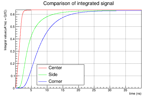
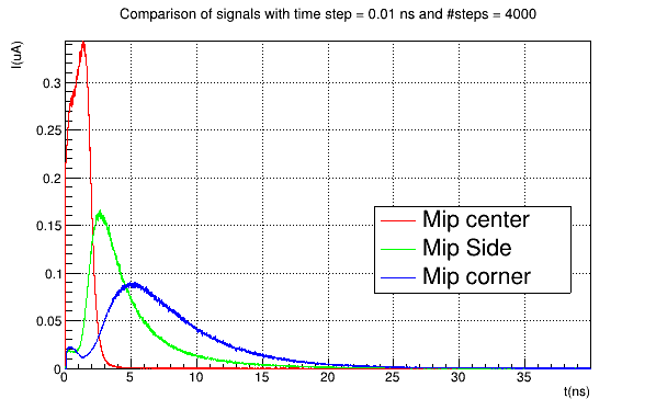
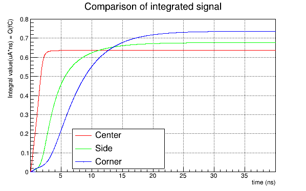
…another thing we could check: how do these plots compare when not looking at the CCE but at the total induced current or the integrated charge? This should allow us to see if we have an issue in the curve itself or its normalization.
Dear @simonspa ,
Thanks for having a look at log files.
About the ElectricFieldReader, we import an electric filed map from TCAD and we use the following configuration:
[ElectricFieldReader]
model = “mesh”
file_name = “iv_50_-2_0.8_nodoping_nosio2_ElectricField.init”
field_scale = 1 1
output_plots = true
output_plots_project = z
output_plots_projection_percentage = 0.99
output_plots_single_pixel = false
So in the end, the electric field will be replicated for all the pixels that make up the matrix.
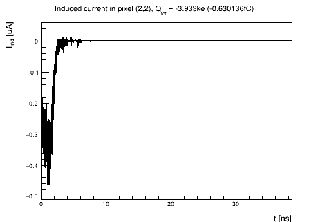
The total induced current plot for the matrix signal and the integrated charge that I obtain are:
Anyway, I can send you by email the configuration files and the maps we’re using.
Thanks a lot!
Chiara
Hi @cferrero
yes, please send me the configs and field maps - I will investigate what’s wrong here.
Simon
Adding this here as reference for others to find it: the problem is double counting appearing at pixel boundaries when a 1x1 induction matrix is used. The fix can be found here:
The first version to include this will be v1.6.2.