Mis-aligned TCAD meshes

[damir]

Hi everybody,

I’ve been trying to simulate the behaviour of a set of deposited charges, under a TCAD simulated electric field and Ramo potential, as well as a constant magnetic field. I’ve recently updated my simulation to use AllPix v3.0.0, and I’ve encountered some behaviour I don’t understand.

I’m trying to simulate a 2D cross-section of a set of 5 silicon strips, each having a 75.5 micron pitch and 304 micron depth. I’ve implemented this setup into allpix as a very simple custom detector:

detectors_file.conf:

[detector1]
type = “prototype_strip”
position = 0 0 0
orientation = 0rad 0rad 0rad

prototype_strip.conf:

type = “monolithic”

number_of_pixels = 1 5
pixel_size = 1um 75.5um
sensor_thickness = 304um

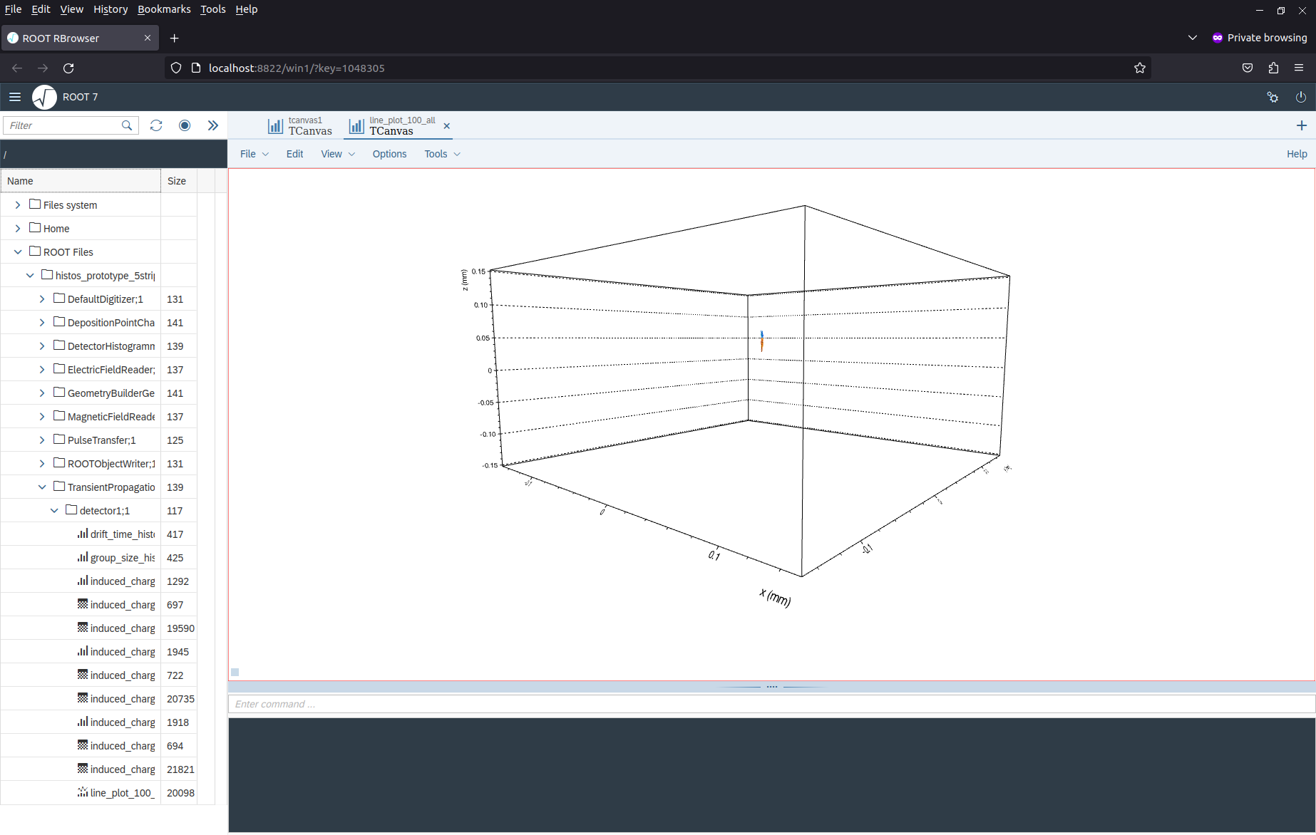
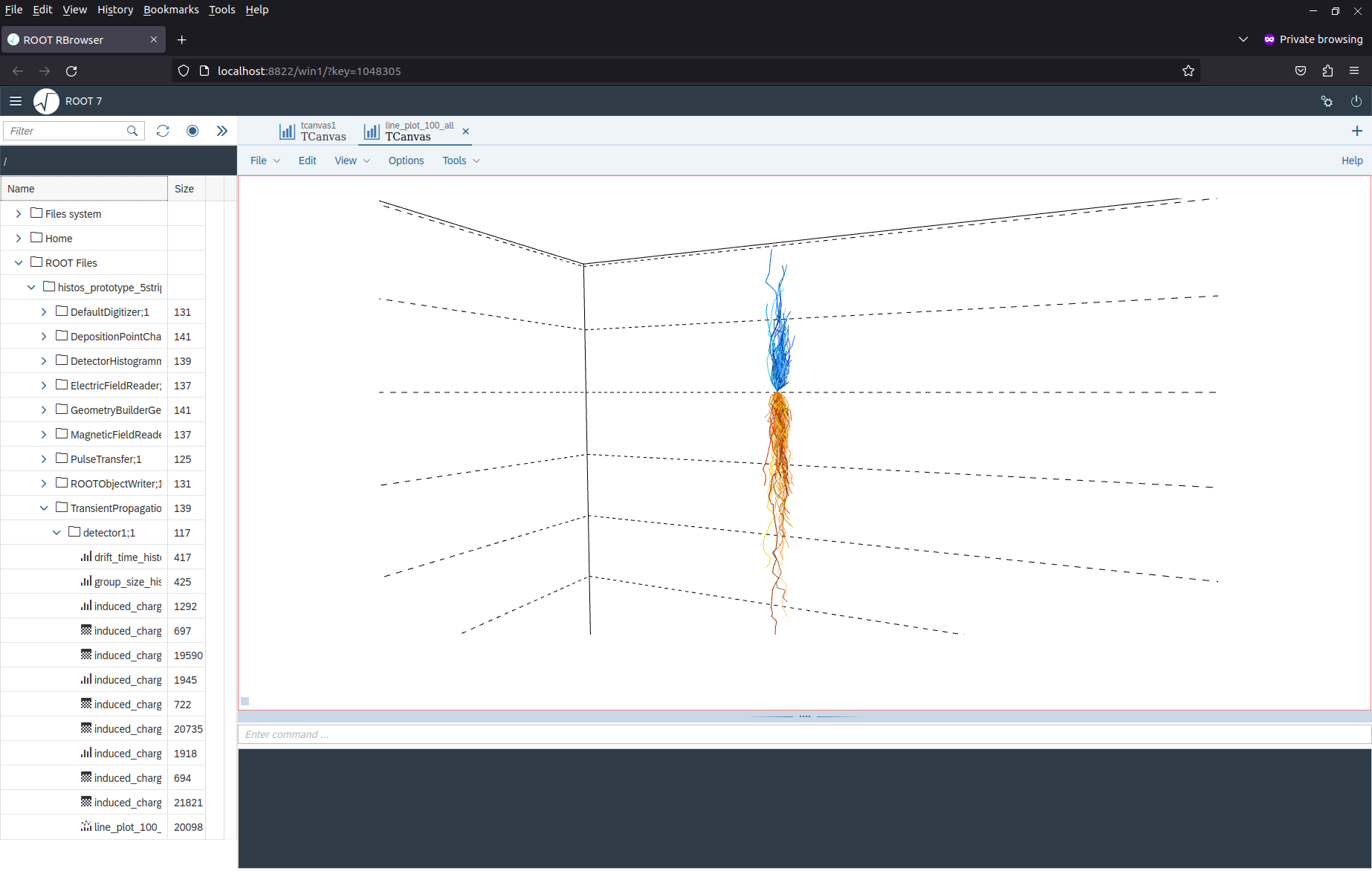
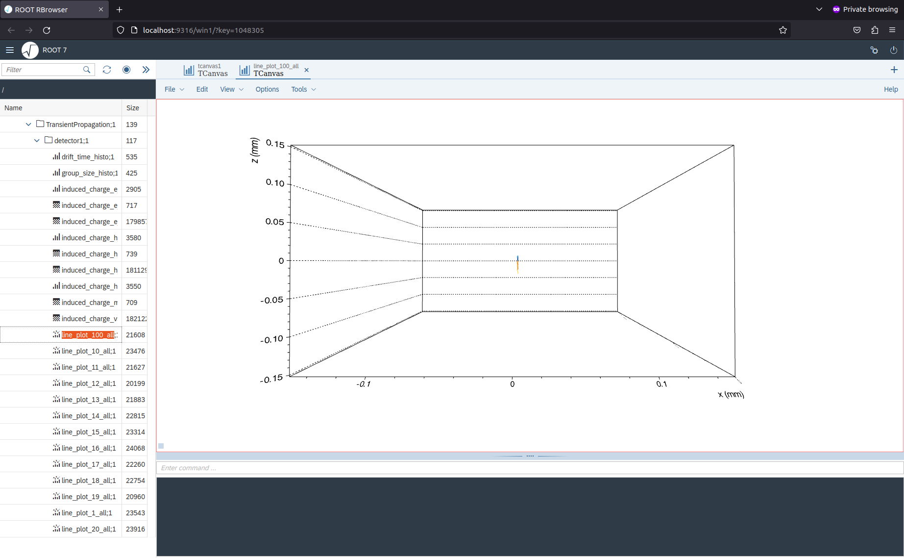
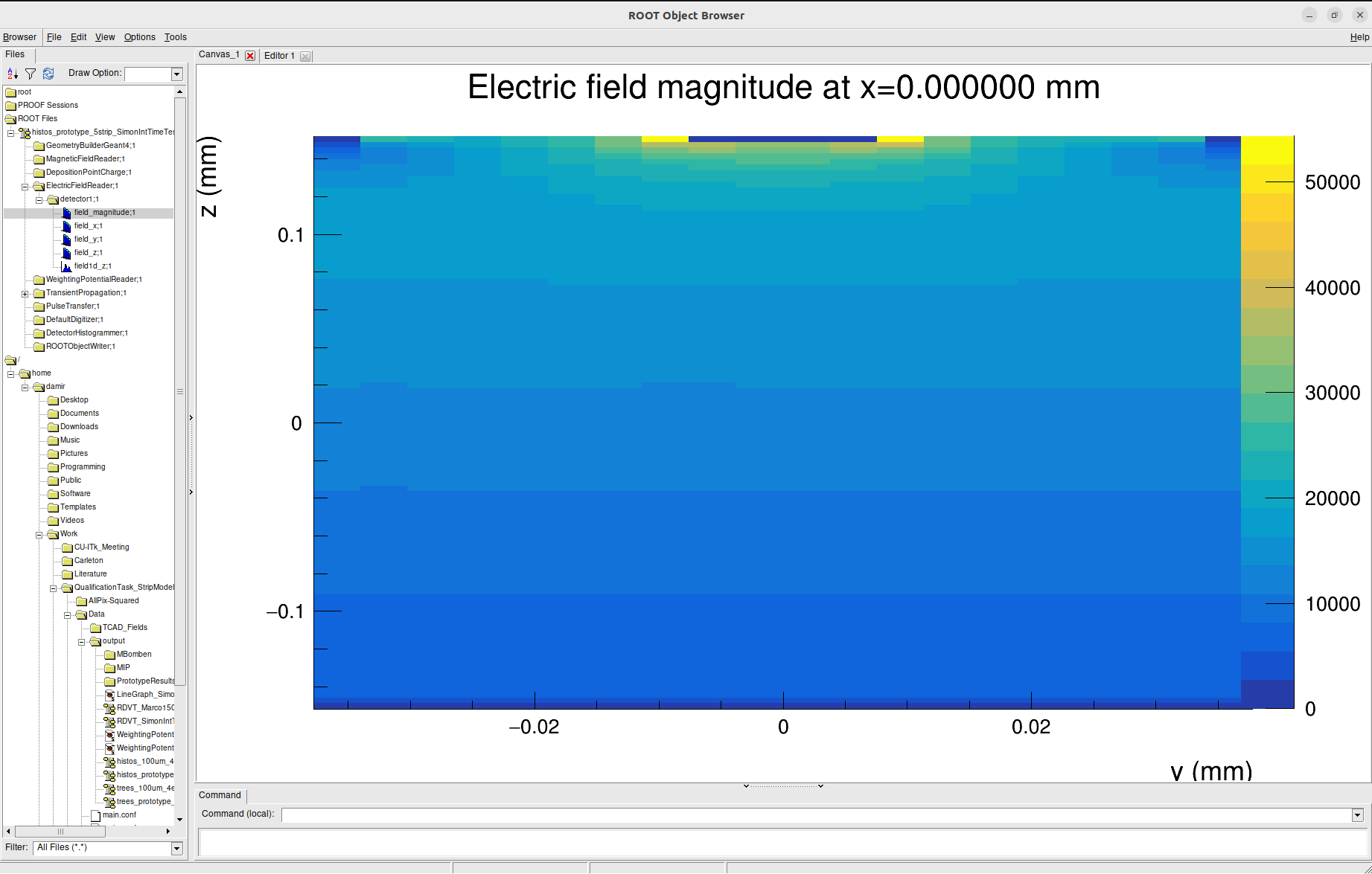
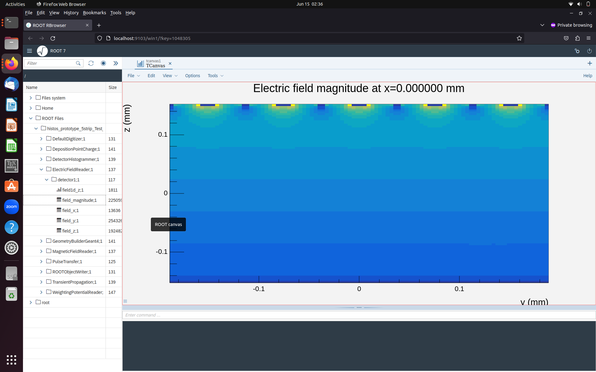
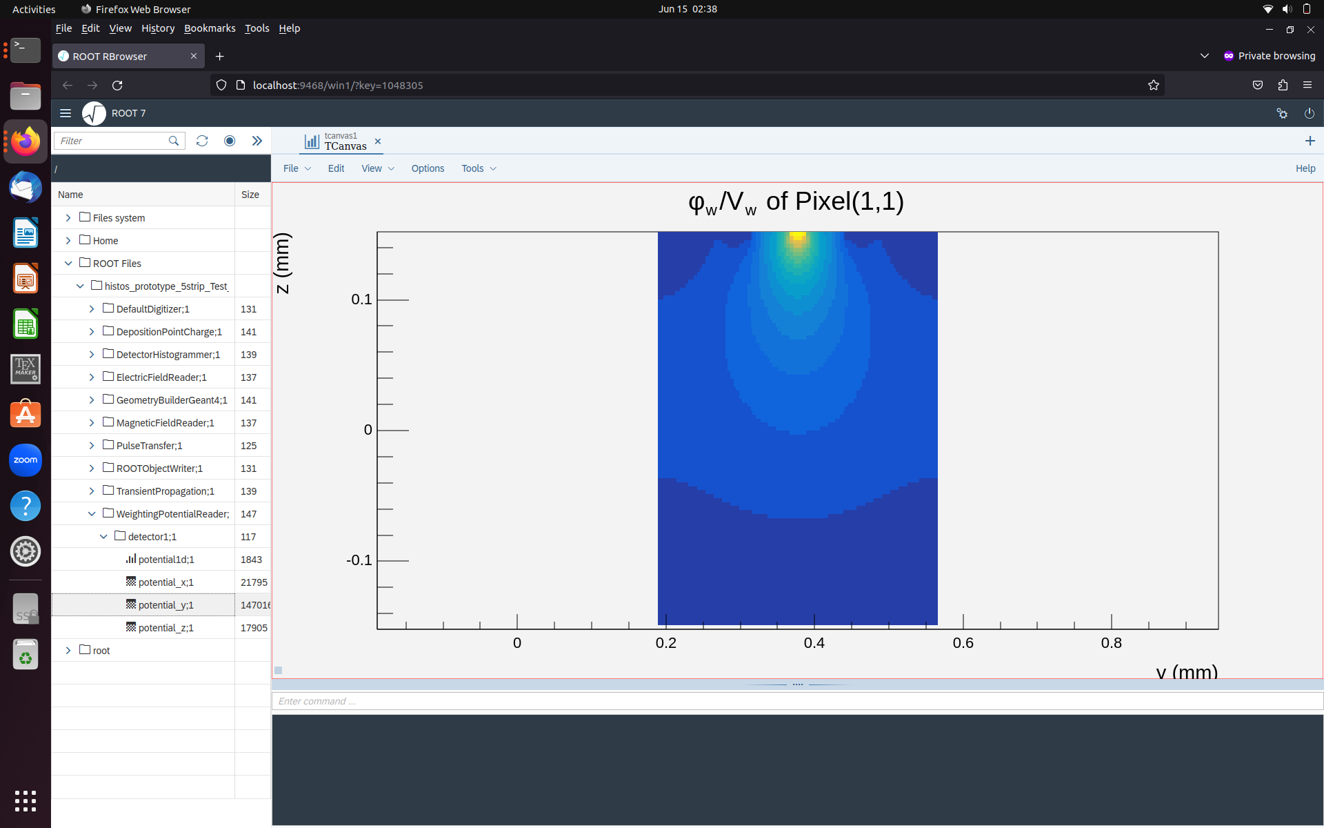
Both my meshes are 377.5 microns wide and 304 microns deep, and I’d expect allpix to fit them into the above detector without issue, but when I look at the fields in the ElectricFieldReader and WeightingPotentialReader histograms, they look strange:

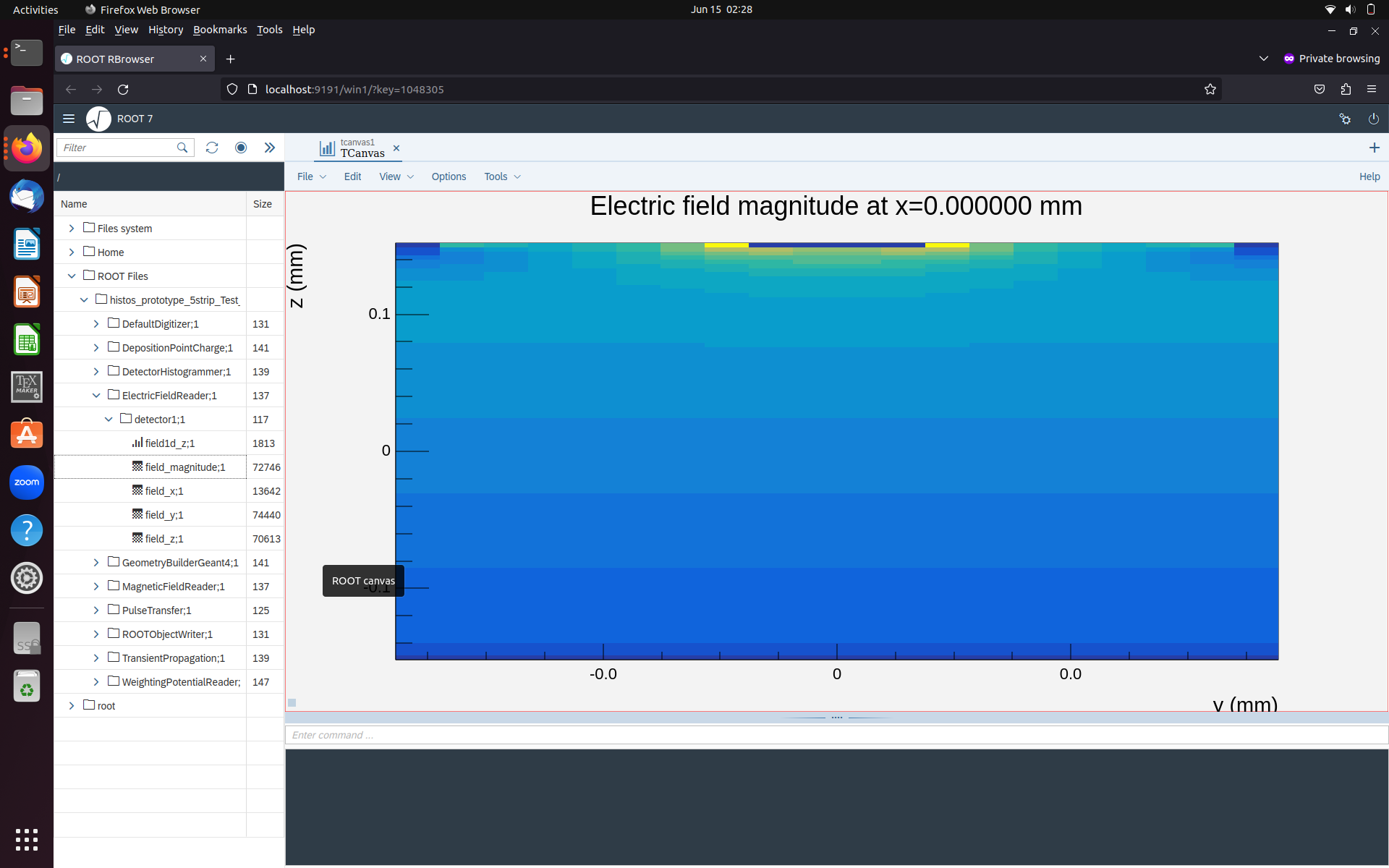
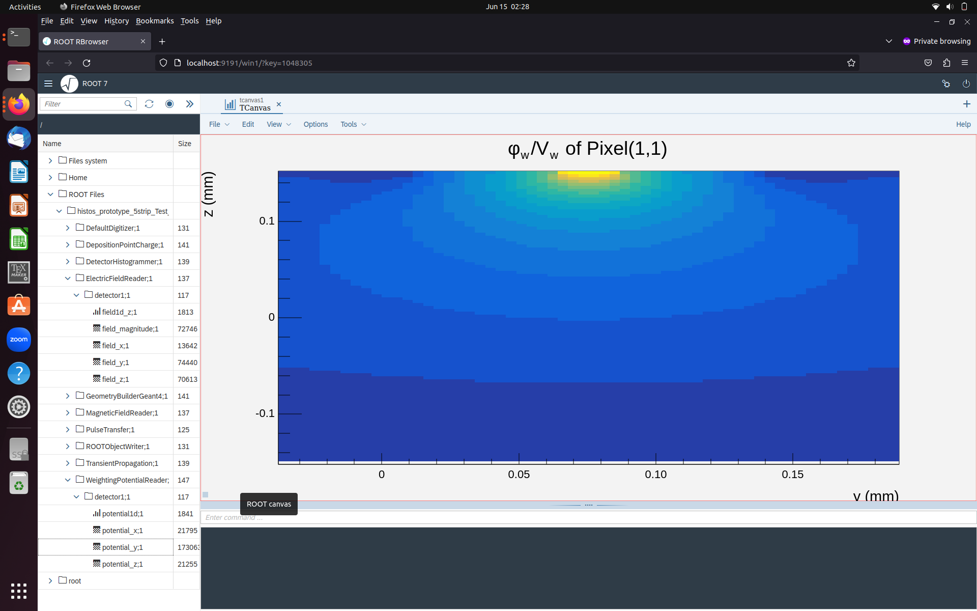
I’m not sure what’s going on here. The electric field map (top) is only one strip wide, where I’d expect it to be 5 strips wide. The weighting potential is 25 microns wide, which doesn’t match the size of anything, but it’s also offset from 0 by about 8 microns or so? I don’t think that should be happening either.

As an experiement, I changed the prototype_strip.conf file to have just one, 377.5 micron wide pixel:

type = “monolithic”

number_of_pixels = 1 1
pixel_size = 1um 377.5um
sensor_thickness = 304um

This results in more weird behaviour:

Now both fields look like what I’d expect them to, but now the weighting potential is offset and sits to the right of the electric field in the space? Shouldn’t they overlap, and both be centred at 0?

Suffice it to say that both of these setups produce unphysical results. The charge collection efficiency that I calculate from these is something like 1%, and I can’t really think of anything else in my configuration that might be causing such a result.

Cheers,
Damir

[simonspa]

Hi @damir

they are not misaligned byt they work differently. The electric field is a static thing placed in the sensor, and whenever an algorithm needs a efield value, it is returned from that position.

Weighting potentials work differently since they need to encode a relative position to an electrode. Hence, the weighting potential is always aligned at the electrode in question, and then the field relative to that position is calculated at the queried point in the sensor. Please have a read, we have a dedicated section in the manual on this:

Field Maps

The plots therefore just shows one configuration of this. We fix the weighting potential to pixel 1,1, for demonstration purposes.

If this doesn’t clarify the situation I’d be more than happy to receive additions to the manual explaining it more clearly.

Cheers,
Simon

[simonspa]

…for answering the other interleaved questions: a crucial input is your module configuration. By default for example, the ElectricFieldReader does not plot your field but it plots one pixel and the field contained within so you can actually check that it aligns well - which seems to be the case in your first image.

[damir]

Hi Simon,

If this doesn’t clarify the situation I’d be more than happy to receive additions to the manual explaining it more clearly.

Yeah, I read through the field map part of the manual when I moved from v2.3.2 to v3.0.0. I’m guessing that this section is a recent addition, since some of grammar seems off and some of the explanations are a bit unclear. I’ll try to recommend some changes throughout the post.

they are not misaligned byt they work differently. The electric field is a static thing placed in the sensor, and whenever an algorithm needs a efield value, it is returned from that position.

Thanks, this conforms to my previous understanding of how allpix uses the E-Field mesh.

…for answering the other interleaved questions: a crucial input is your module configuration. By default for example, the ElectricFieldReader does not plot your field but it plots one pixel and the field contained within so you can actually check that it aligns well - which seems to be the case in your first image.

Thanks for the clarification. For reference, in the above plots I used ’ field_mapping = “SENSOR” '. I did this since my TCAD mesh is the same size as the detector model I made (377.5um wide and 304um deep). I’m guessing that the periodic application mentioned in the “SENSOR” documentation refers to a case where the TCAD mesh is only the size of a single pixel, and it needs to be placed in each of the pixels in the model file.

Weighting potentials work differently since they need to encode a relative position to an electrode. Hence, the weighting potential is always aligned at the electrode in question, and then the field relative to that position is calculated at the queried point in the sensor. Please have a read, we have a dedicated section in the manual on this:

I think I understand what the manual is saying, but just to put it in my own words:

Each pixel has an electrode on it, and each electrode has a charge induced on it when charges carriers move through the pixel. To calculate the induced charge on a given electrode, the Weighting Potential needs to be moved so that it is centred on that electrode. This process is repeated for each electrode.

This sort-of explains the Weighting Potential plot (the second image) in the OP. The field is centred at approximately 0.075mm, which is one pixel pitch to the right of the origin. I’m guessing when you said:

The plots therefore just shows one configuration of this. We fix the weighting potential to pixel 1,1, for demonstration purposes.

You’re just saying that this is the position that was chosen for the purposes of generating this plot, and the choice is arbitrary, since any pixel (except perhaps the edge pixels?) could’ve been used for the same thing.

Some follow-up questions:

The weighting field in the image seems to be around 240um wide. I’m guessing this is also a result of some decision around what to show on the plot? For reference, my config file has the following:

[WeightingPotentialReader]
model = “mesh”
file_name = “TCAD_Fields/fields_5strip_des_WEIGHTINGPOTLONLY_WeightingPotential.init”
field_mapping = “PIXEL_FULL”
ignore_field_dimensions = true
output_plots = 1

Additionally, I’m curious about how allpix handles pixel “grids” that only have one pixel in the x-dimension. Since I’m simulating strips, my pixel grid is 1x5 and all my Weighting Potentials are 2D. Is there anything I have to consider when using 2D Weighting Potentials apart from the “ignore_field_dimensions” line in the config file there?

The reason I’m asking is that I’ve recently been trying to calculate some charge collection efficiencies for my configuration and they’re much lower than expected for the fluence that I’m using (something like 1/25th of what I expect). I’m trying to figure out whether something is wrong with the Weighting Potentials, something that might affect the CCE calculation in a negative way.

Regards,
Damir

[simonspa]

Hi @damir

@damir

I’m guessing that the periodic application mentioned in the “SENSOR” documentation refers to a case where the TCAD mesh is only the size of a single pixel, and it needs to be placed in each of the pixels in the model file.

Yes, or multiple pixels, or a fraction of a pixel - all these will work. Very often, pixel sensors are organized in double columns with differences also in the e-field between even and odd columns. In cases like this, the SENSOR mapping provides the necessary flexibility.

@damir

Each pixel has an electrode on it, and each electrode has a charge induced on it when charges carriers move through the pixel.

Well, almost. Eevery pixel may have multiple electrodes. Also, induced current is also calculated when charge carriers move through adjacent pixels (see distance parameter).

@damir

You’re just saying that this is the position that was chosen for the purposes of generating this plot, and the choice is arbitrary, since any pixel (except perhaps the edge pixels?) could’ve been used for the same thing.

Exactly correct.

@damir

The weighting field in the image seems to be around 240um wide. I’m guessing this is also a result of some decision around what to show on the plot?

The plot should show three adjacent channels, i.e. the width should be 3*pitch = 226.5um for you.

@damir

I’m curious about how allpix handles pixel “grids” that only have one pixel in the x-dimension. Since I’m simulating strips, my pixel grid is 1x5 and all my Weighting Potentials are 2D. Is there anything I have to consider when using 2D Weighting Potentials apart from the “ignore_field_dimensions” line in the config file there?

If you really only have strips, i.e. a single row of pixels, this is all you need. The check and setting is there to prevent people using 2D weighting potentials on a 3D pixel grid - which will generate a perpetuum mobile since the same current would be induced on all pixels in the column.

@damir

I’m trying to figure out whether something is wrong with the Weighting Potentials, something that might affect the CCE calculation in a negative way.

Do you get reasonable/expected results when not including radiation damage?

Best,
Simon

[damir]

Hi Simon,

Do you get reasonable/expected results when not including radiation damage?

Not really. I recently tried to reduce the fluence by a factor of 1000, but I still get a charge collection efficiency of something like 2.8%. My TransientPropagation module:

#Using Transient Propagation since it uses the Ramo-Schokley Theorem
[TransientPropagation]
temperature = 253K
charge_per_step = 10
mobility_model = “canali”
trapping_model = “cmstracker”
fluence = 1e12/cm/cm
distance = 2
output_plots = 1
output_linegraphs = true

For reference, I used to set the fluence to “4e15/cm/cm”.

The charges just aren’t moving enough to induce the charge that I expect. If you look at a linegraph I used to debug, you can see the charges have very limited movement:

If I zoom in:

The total movement is something like 25 microns.

Regards,
Damir

[simonspa]

Hi @damir

Reducing it to 1e15 is not n"switching it off!

I want to see how things behave completely without trapping, since this is e.g. also influenced by your doping concentration that might be miles off. Maybe post or attach your full config files for reference instead of just snippets.

But looking at line graphs certainly is a very good idea!

Cheers,
Simon

P.S. it is very convenient to enclose config snippets in tripple-backtick blocks (```) and if you want to get fancy, adding highlighting by adding ini directly after the opening backticks

[damir]

Hi Simon,

@simonspa

Reducing it to 1e15 is not n"switching it off!

I want to see how things behave completely without trapping, since this is e.g. also influenced by your doping concentration that might be miles off. Maybe post or attach your full config files for reference instead of just snippets.

Sorry, I thought that reducing the fluence to 1e12 would do what I wanted. I’ve set the “trapping_model” parameter to “none”. Here is the full config file:

[Allpix]
log_level = "WARNING"
log_format = "DEFAULT"
model_paths = "/eos/user/d/damir/ALLPIX2_Remote/Prototype/Configurations"
detectors_file = "Configurations/detectors_file.conf"
number_of_events = 100
root_file = "histos_prototype_5strip_SimonNoTrap"
random_seed = 0

#The geometry is empty for now
[GeometryBuilderGeant4]

#Magnetic Field Reader
[MagneticFieldReader]
model = "constant"
magnetic_field = 0T 2T 0T

#Depositing the charges directly
[DepositionPointCharge]
#Fixed-point model
source_type = "point"
model = "fixed"
position = 0um 151um 0um
number_of_charges = 1000
output_plots = 1

#Electric Field Reader
[ElectricFieldReader]
model = "mesh"
file_name = "TCAD_Fields/fields_5strip_des_ElectricField.init"
field_mapping = "SENSOR"
output_plots = 1

#Ramo Potential Reader
[WeightingPotentialReader]
model = "mesh"
file_name = "TCAD_Fields/fields_5strip_des_WEIGHTINGPOTLONLY_WeightingPotential.init"
field_mapping = "PIXEL_FULL"
ignore_field_dimensions = true
output_plots = 1

#Using Transient Propagation since it uses the Ramo-Schokley Theorem
[TransientPropagation]
temperature = 253K
charge_per_step = 10
mobility_model = "canali"
#TEST: Removing Charge Trapping
trapping_model = "none"
#trapping_model = "cmstracker"
fluence = 1e12/cm/cm
#The newest version of allpix (v3.0.0) uses something called "distance" instead of an induction matrix
distance = 2
output_plots = 1
output_linegraphs = true

#Pulse Transfer
[PulseTransfer]
max_depth_distance = 5um
output_plots = 1

#Default Digitizer
[DefaultDigitizer]
threshold = 1e
output_plots = 1

#Detector Histogrammer
[DetectorHistogrammer]

#Define the .root file that contains the tree, and what leaves the tree contains
[ROOTObjectWriter]
file_name = "trees_prototype_5strip_SimonNoTrap"
include = "MCTrack","MCParticle","PixelCharge","PixelHit","PropagatedCharge","DepositedCharge"

Wow, the code looks much better in the triple-single-quotes.

Suspiciously, changing this doesn’t really affect the results I get. Before I changed this, I got a charge collection efficiency of ~2.82%, and after the change it’s around 2.8%. So the simulation is different, but not significantly.

If I plot the line graphs, we once again see a lack of movement:

I don’t think the doping concentration is the issue here, if only because that’s something I haven’t really thought about, and I assume that it’s handled in some way in the TCAD meshes.

Cheers,
Damir

[simonspa]

Hi @damir

@damir

Wow, the code looks much better in the triple-single-quotes.

Indeed it does

@damir

I don’t think the doping concentration is the issue here

Nope, since you don’t define any.

Could you re-run the same simulation setting also

[TransientPropagation]
integration_time = 250ns

and then look again at the line graph?

(or on the command line without editing your configs: allpix -c config.conf -o TransientPropagation.integration_time=250ns)

I am wondering if your charge collection is just very slow, and your plots above don’t contain a color axis label for the electric fields, so I don’t know how strong it is.

Cheers,
Simon

[damir]

Hi Simon,

First thing’s first, I tried the intergration_time change. My [TransientPropagation] module now looks like this:

#Using Transient Propagation since it uses the Ramo-Schokley Theorem                                                                                                                                       
[TransientPropagation]
temperature = 253K
charge_per_step = 10
mobility_model = "canali"
#TEST: Removing Charge Trapping                                                                                                                                                                            
trapping_model = "none"
#trapping_model = "cmstracker"                                                                                                                                                                             
#fluence = 4e15/cm/cm                                                                                                                                                                                      
fluence = 1e12/cm/cm
#The newest version of allpix (v3.0.0) uses something called "distance" instead of an induction matrix                                                                                                     
distance = 2
#induction_matrix = 1 1                                                                                                                                                                                    
integration_time = 250ns
output_plots = 1
output_linegraphs = true

Unfortunately, it doesn’t have much of an effect. A random line graph:

The CCE is also only slightly different from what it used to be (something like 2.9% compared to 2.8%).

@simonspa

I am wondering if your charge collection is just very slow, and your plots above don’t contain a color axis label for the electric fields, so I don’t know how strong it is.

I was thinking something similar; maybe I’m not running the simulation for long enough and so there isn’t enough time for charge to be induced on the electrodes?

Speaking of my fields now having a colour axis, this has also bothered me. Is there any way to force allpix to print them? I’m thinking that it’s something that you have to use a macro once you have the .root file.

Cheers,
Damir

[simonspa]

@damir

maybe I’m not running the simulation for long enough

That’s exactly what the integration_time parameter is for. You just extended the simulation time by a factor 10 with little impact.

@damir

Is there any way to force allpix to print them?

This is an issue with ROOT, not Allpix Squared, the axis are there but somehow not displayed using this webbrowser thingy. Try opening the files with root --web=off?

How does the log of a single event look like on DEBUG level? Just rerun with allpix -c config -v DEBUG -o number_of_events=1

If this doesn’t help us, I might have to look into your simulation a bit deeper, for which I would need your config files and fields.

Best,
Simon
/Simon

[damir]

Hi Simon,

@simonspa

This is an issue with ROOT, not Allpix Squared, the axis are there but somehow not displayed using this webbrowser thingy. Try opening the files with root --web=off?

You were right. I was using the web-browser version since it more easily allows manipulating the 3D line graphs. If I do it the old-fashioned way, it looks like this:

It’s still not the best, I had to shift the colour-axis to the left a bit to fit the numbers on the screen. In general the electric field scales from “0” to “50000”. To be honest, I’m not sure how to interpret these values. According to the .init file make of the electric field, the field units are “V/cm”

Allpix Squared v3.0.0 TCAD Mesh Converter, observable: ElectricField
V/cm ##EVENTS##
##TURN## ##TILT## 1.0
0.0 0.0 0.0
304 1 377.5 0.0 0.0 0.0 0.0 1 100 100 0.0

This is chosen by me in my mesh_converter config file (observable_units = V/cm). However, looking at the actual values in the .init file, I can’t really see many above (-)18,000. Is an electric strength of ~25,000 V/cm even physically plausible in a small strip like this?

That question aside, I actually tried to mess with my .init file a bit to see if I could change the field strength and potential get more charge movement. I basically just changed the V/cm listed above into something like kV/mm, which should result in a much stronger field. Unfortunately, allpix is a bit too smart, and decides to interpret the field as V/cm against my wishes. Is there a way to force allpix to accept the listed units in the .init file? Or better yet, force it to interpret the values in the .init file as having units of my choosing?

@simonspa

How does the log of a single event look like on DEBUG level? Just rerun with allpix -c config -v DEBUG -o number_of_events=1

I piped the stdout and stderr into a .txt file after implementing those verbosity and event number changes into the config file. I’ve attached the .txt file below. I haven’t been able to look at it in detail yet, but it seems that (at least for this event) the charges bounce between y=150um and y=152um. They seem to be almost stuck where they started, even though the you can see the trapping being turned off earlier in the output.

AllPix_TestOutput.txt (164.8 KB)

Cheers,
Damir

[simonspa]

@damir

To be honest, I’m not sure how to interpret these values.

If you’re shifting further (intricacies of ROOT plotting) you’ll also see the axis has a label:

@damir

I piped the stdout and stderr into a .txt file after implementing those verbosity and event number changes into the config file.

allpix -l file.txt woudl have been another option.

Looking at the file I think I found the flaw:

Wrapper dimensions of model: (1um,377.5um,304um)

You defined your detector as being 1um “long” (along your strip dimension). This does not work in Allpix Squared since we always perform 3D simulations. So as soon as your charge carriers start moving, they will hit a sensor wall (of the 1um strip length) and are stopped.

Even when using 2D field maps, your strip length should be the correct length of your detector, likely multiple millimeters. The field is then just “stretched” in that direction.

Cheers,
Simon

[damir]

Hi Simon,

I’m happy to report that your suggestion to extend the “length” of the strip worked fantastically. I extended the detector to have a length of 500 microns and all the charges move fairly freely now. If I deposit the charges at z=0 (around 150 microns from the electrode), the line graphs look like this:

Additionally, the charge collection efficiency I calculate from this scenario is much more normal, being something like 87%.

I am wondering about some of the new output I’m getting when I run this:

[damir@lxplus750 Prototype]$ allpix -c main.conf
|07:18:34.726|  (STATUS) Welcome to Allpix^2 v3.0.0
|07:18:34.727|  (STATUS) Initialized PRNG with configured seed 0
|07:18:55.295|  (STATUS) Loading module DepositionPointCharge
|07:18:55.947| (WARNING) Model file "/eos/home-d/damir/ALLPIX2_Remote/Prototype/Configurations/prototype_strip.conf" does not provide a geometry parameter, using default
|07:18:55.957|  (STATUS) Loading module TransientPropagation     
|07:18:55.958| (WARNING) [C:TransientPropagation:detector1] Per-event line graphs or animations requested, disabling parallel event processing
|07:18:55.958| (WARNING) Module instance TransientPropagation:detector1 prevents multithreading
|07:18:56.032|  (STATUS) Loaded 10 modules                   
|07:18:56.032|   (ERROR) Multithreading disabled since the current module configuration does not support it
|07:18:56.032|  (STATUS) Initializing 10 module instantiations
|07:18:58.705| (WARNING) [I:ElectricFieldReader:detector1] Field map size is (1um,377.5um) but expecting a multiple of the pixel pitch (500um, 75.5um)
                                                           The area to which the field is applied can be changed using the field_scale parameter.
|07:18:59.160| (WARNING) [I:WeightingPotentialReader:detector1] No field units provided, interpreting field data in internal units, this might lead to unexpected results.
|07:18:59.162|   (ERROR) [I:WeightingPotentialReader:detector1] Requesting to interpret INIT field as units "" while file header states "V"
|07:18:59.167| (WARNING) [I:WeightingPotentialReader:detector1] Weighting potential with 2 dimensions detected, requiring three-dimensional scalar field - this might lead to unexpected behavior.
|07:18:59.167| (WARNING) [I:WeightingPotentialReader:detector1] Field map size is (1um,377.5um) but expecting a multiple of the pixel pitch (500um, 75.5um)
                                                                The area to which the field is applied can be changed using the field_scale parameter.
Warning in <TH1::TH1>: nbins is <=0 - set to nbins = 1
Warning in <TH2::TH2>: nbinsy is <=0 - set to nbinsy = 1
|07:18:59.696|  (STATUS) Initialized 10 module instantiations
|07:18:59.697|  (STATUS) Starting event loop
|07:19:38.366|  (STATUS) Finished run of 100 events             
|07:19:39.103|  (STATUS) [F:ROOTObjectWriter] Wrote 21127 objects to 7 branches in file:
                                              /eos/home-d/damir/ALLPIX2_Remote/Prototype/output/trees_prototype_5strip_PrelimResults150.root
|07:19:39.376|  (STATUS) Finalization completed
|07:19:39.377| (WARNING) Unused configuration keys in section DepositionPointCharge:detector1:
                         output_plots
|07:19:39.378|  (STATUS) Executed 10 instantiations in 43 seconds, spending 83% of time in slowest instantiation TransientPropagation:detector1
|07:19:39.378|  (STATUS) Average processing time is 386.696ms/event, event generation at 3 Hz

It’s complaining about the 2D weighting potential, even though I tell it to ignore the field dimensions, but that’s happened before and not really important. It’s also complaining that my field map size is not a multiple of the pixel pitch. I suspect that allpix is smart enough that this isn’t causing problems; I’m guessing that it does something like place the full field map across all 5 pixels at every possible x value. If it doesn’t work like this, please let me know.

Cheers,
Damir

[simonspa]

Hi @damir

@damir

I suspect that allpix is smart enough that this isn’t causing problems; I’m guessing that it does something like place the full field map across all 5 pixels at every possible x value.

It works exactly as you describe, the warning comes from the other dimension, where 1um != 500um. But since you knowingly and willingly (and sensibly ) load 2D field maps, that is alright!

Happy simulation,
Simon