MCParticle vs MCtrack energies

Hi,
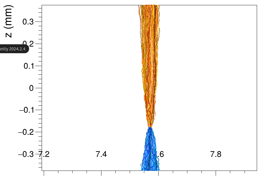
For my purpose i need to retrieve the true interactions positions of gamma rays interacting with a silicon detector as well as the deposited energies. For this reason i was playing around with MCTrack and MCParticle. The simulation consists in 2 point sources, 9 cm away from the detector surface.
Although i though MCTrack was enough for this purpose i thought of having a look anyway at MCParticle but i found some discrepancies and unexpected behaviors and i am not sure if those arise from errors in the allpix functions or from my understanding of them.

Using a python script i was getting data from MCTrack and MCParticle as

        for mc_track in br_mc_track:
        #here we record all the interactions the event had with the detector togheter with the tracks generated
        data_array[1] = mc_track.getStartPoint().x()
        data_array[2] = mc_track.getStartPoint().y()
        data_array[3] = mc_track.getStartPoint().z()
        data_array[4] = mc_track.getGlobalStartTime()
        data_array[5] = mc_track.getKineticEnergyInitial()
        data_array[6] = mc_track.getCreationProcessName()
        data_array[7] = mc_track.getParticleID()
        data_array[8] = hex(ROOT.addressof(mc_track))
        data_array[9] = hex(ROOT.addressof(mc_track.getParent()))
        data_array[10] = mc_track.getOriginatingVolumeName()

        # Create a dictionary from the array and column names
        new_row = dict(zip(df.columns, data_array))
        print(iev)

        # Convert the dictionary to a DataFrame and append it
        df = pd.concat([df, pd.DataFrame([new_row])], ignore_index=True)

    for mc_particle in br_mc_particle:
        data_array[1] = mc_particle.getGlobalStartPoint().x()
        data_array[2] = mc_particle.getGlobalStartPoint().y()
        data_array[3] = mc_particle.getGlobalStartPoint().z()
        data_array[4] = mc_particle.getGlobalTime()
        data_array[5] = mc_particle.getKineticEnergyStart()
        data_array[6] = f"mc_particle, is it primary? {mc_particle.isPrimary()}. Connected track: {hex(ROOT.addressof(mc_particle.getTrack()))}"
        data_array[7] = mc_particle.getParticleID()
        data_array[8] = hex(ROOT.addressof(mc_particle))
        data_array[9] = hex(ROOT.addressof(mc_particle.getParent()))
        data_array[10] = "parent particle: {hex(ROOT.addressof(mc_particle.getPrimary()))}"

        new_row = dict(zip(df.columns, data_array))
        print(iev)

        df = pd.concat([df, pd.DataFrame([new_row])], ignore_index=True)

respectively where iev is the event ID.

An example of results is shown below

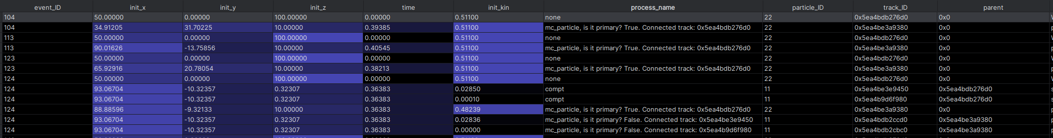
We can see that for event IDs 104,113,123 everything looks fine, the first row(s) in each event are from MCTrack, and the initial kinetic energy (init_kin) is 511 keV as set in the .conf file for the source. the same is shown in the MCParticle row(s), with the difference that the initial coordinates are in proximity with the detector surface (which is at z=0) since MCParticle start saving informations of the particle once this enters the detector.

But then when we start to have interactions in the active area of the detector as for event 124, in the MCParticle rows (distinguishable from having mc_particle under the column process_name), we see that the starting kinetic energy of the primary particle is not 511 kev as expected but lower like 482keV.
If we look at the deposited energy from the first compton interaction by summing the initial kinetic energy of the secondary particles related to the interaction we notice that 482keV should rather be the energy of the primary particle after the interaction (so after having deposited some of its energy since 511-28.36=482.64keV).

Similarly happens for all other cases in which there is an interaction in the detector, where the init_kin from MCParticle is lower than 511kev and very similar to the final energy of the primary particle after having interacted.

On a last note if i calculate the deposited energy in the compton interaction looking at MCTrack for event 124, i would sum 28.5keV+0.1keV=28.6keV, while from MCParticle= 28.36keV+0.0keV =28.36keV. Similarly for all other interaction cases the results seem to be slightly different. Could this be because MCParticle looks at the true deposited energy while MCTrack has the true deposited energy + other effects present in the physics model such as doppler broadening? (i am using FTFP_BERT_PEN)

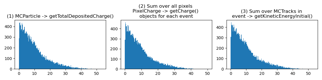
I also looked at getTotalDepositedCharge() for MCParticle and from that divide by 2 and multiply by 3.64eV and i do get similar results as from the other two ways mentioned before to measure the deposited energy although not exactly the same and i am not sure what is the more accurate/best way among those 3.

Bests

Luca

TLDR: if i want to know the deposited energy by a photon having a compton scattering or photoabsorption in the detector should i look at MCTrack initial kinetic energies of the secondaries, MCParticle initial kinetic energies of the secondaries, or MCParticle deposited charge of primary and secondaries? (or is it all the same?)

Hi @luca_tero

I would again say that it depends on what you’d like to do with these numbers. Would you like to know how much …

  • energy the primary lost?
  • energy the secondary particle had?
  • energy was deposited?
  • charge was deposited?

It’s different steps of the simulation, so of course there are minor differences. The difference between lost and secondary/deposited energy could be correlated with e.g. ionisation energy. The deposited charge again is somewhat randomised and undergoes rounding, see here.

Thus, I believe it is really up to you and your research goal which observable to choose. One thing that I would like to clarify, however:

  • MCTrack is an object recording a particles (regardless of being primary/secondary) properties through the full setup.
  • MCParticle is an object recording a traversal of an MCTrack through an individual sensitive volume. This is the reason why it starts just at the surface of your sensor and can already have a different initial energy than the MCTrack, because it’s the energy the particle had when entering the sensor.

Cheers
Paul

Hi

Thank you for the clarification. My interest is knowing the true energy deposited in the detector (which later on in a more realistic setting i will change and calculate it from the charge deposited)

Regarding MCParticle starting kinetic energy i understand the concept you mean but from my simulations i found that whenever the primary photon interacts with the active volume of the detector (and not before since there is nothing else before it, not even passive volumes and i set all in vacuum), then the kinetic initial energy from MCParticle for the primary photon at the point of entrance of the detector is lower than the energy of the monochromatic source (511 keV). This happen on all such cases.

On the contrary for all cases in which the primary photon does not interact with the detector the MCParticle kinetic initial energy signaled at the entrance of the detector is 511 keV.

But i’ll check better for that in case i made some mistakes in the conf or in the python code to read the ROOT file.

Bests

Luca

Hi @luca_tero ,

I do understand the issue, yes. I could imagine that Geant4 only emits a new “step” when the actual interaction is taking place, such that then at the beginning of this new step the energy was already decreased. I know that we distinguish photons from other particles when it comes to the position of the deposit, maybe we also have to adapt this part.

Would you mind providing us with your configurations, such that we can reproduce and investigate the issue?

Thanks!
Paul

Hi

Sure thing, here is the main conf file i use:

[Allpix]
log_level = "INFO"
log_format = "DEFAULT"
detectors_file = "detector.conf"
number_of_events = 10000

[GeometryBuilderGeant4]
world_material = "vacuum"


[DepositionGeant4]
record_all_tracks= true
physics_list = FTFP_BERT_PEN


source_type = "macro"
file_name = "Source_test.mac"


number_of_particles = 1
max_step_length = 0.5um
range_cut = 3.0um

#[ElectricFieldReader]
[Ignore]
model = "linear"
bias_voltage = -100V

#[GenericPropagation]
[Ignore]
temperature = 293K
charge_per_step = 100

#[SimpleTransfer]
[Ignore]
max_depth_distance = 5um

#[DefaultDigitizer]
[Ignore]
threshold = 600e

#[DetectorHistogrammer]


[VisualizationGeant4]
mode = "gui"
accumulate = true
display_trajectories = true
draw_hits = true

[ROOTObjectWriter]
file_name = "ROOT_test_2source.root"
#include = "MCParticle" "MCTrack" "DepositedCharge"


where source_test.mac is

# Point Source 1
/gps/source/intensity 5.
/gps/particle gamma
/gps/pos/type Point
/gps/pos/centre 0.0 0.0 100.0 mm
/gps/ene/type Mono
/gps/ene/mono 511 keV
/gps/ang/type iso


# Point Source 2
/gps/source/add 10.
/gps/particle gamma
/gps/pos/type Point
/gps/pos/centre 50.0 0.0 100.0 mm
/gps/ene/type Mono
/gps/ene/mono 511 keV
/gps/ang/type iso


and detector.conf is of a custom type placed in position and orientation 0 0 0 as follow

type = "monolithic"
geometry = "pixel"

number_of_pixels = 2000 2000
pixel_size = 50um 250um

sensor_thickness = 2cm #just to play around for now and have enough thickness to detect many events

chip_thickness = 100 um

to read the data i then used a custom made python script using the root and allpix libraries, i can provide that too if needed (but nothing fancier than what is already in the allpix example using mc_particle.getKineticEnergyStart() and similar).

also to confirm my understanding, if one would be interested in the ground truth energy deposited in the detector in an interaction then the MCTrack information on the energies would be a good way, while if one wants to look at the energy that the detector will “detect” from that interaction i should look at the deposited charge (for example with MCParticle getTotalDepositedChage), correct?

Bests

Hi @luca_tero ,

I didn’t yet have the chance to work with your examples (busy times here, I’m sorry), but I have an answer to your question:
I did notice that our implementation of an MCParticle does not carry the truth information of deposited energy, but only of deposited charge (with this conversion in between). Hence, at the moment it is quite tricky to get this information, to be honest. I got inspired and am working on an implementation to access this information already, though. Indeed the best estimate you can get at the moment is the energy of the MCTrack or the MCParticle entering the detector.

What you can get from the MCParticle though is the total deposited charge via getTotalDepositedCharge(), exactly as you mentioned.

I will let you know as soon as I have an implementation ready or been able to reproduce your issue above.

Cheers
Paul

Hi @pschutze ,

I see, no worries at all and thank you for your remarks, i will therefore use MCTrack to sum the initial energies of the secondary particles generated by a primary particle interaction in order to approximate the deposited energy, which for what i have to do is enough i would say.

I have no big experience but if there is anything i can do to help in that regard let me know, bests

Luca

Hi @luca_tero ,

I have added a functionality to the MCParticle to store/obtain the total deposited energy, it’s currently under review, in case you’re interested: Add total deposited energy to MCParticle (!1144) · Merge requests · Allpix Squared / Allpix Squared · GitLab

You could test this branch already for your purposes and use the new command MCParticle::getTotalDepositedEnergy().

Cheers
Paul

Hi @pschutze ,

Thank you i am playing around with it and seems to work quite well, ill update if i find any problems on it.

As a side note the problem mentioned here still persist.
Consider for example a photon from a monochromatic source of 511 keV interacting with the detector (and the detector only) once, in which interaction the photon loses 200 kev (generating a secondary recoil electron with that much initial K energy).
The initial kinetic energy obtained from the object MCParticle for the primary photon will not start at 511 kev but rather at 311 keV. This happens despite the fact that the interction takes place deep down in the detector, so that MCParticle initial kinetic energy should still start at 511 keV since this is the energy of the photon when it enters the detector.
On the other hand if the primary photon does not interact at all with the detector, but passes through it, the initial kinetic energy from MCParticle will agree with the one from MCTrack. Related problems occur for some electron tracks as well from what i saw.

It is just a minor detail that does not affect my simulation, but just pointing it out. In the following days i can try to have a look in the code of MCParticle and see from where the problem could arise.

Bests

Luca

Hi @pschutze,

@luca_tero, I’m going to piggyback on your post since I am also seeing something similarly peculiar in regards to the deposited energy.

So I am simulating a silicon xray detector, and only looking at the events that interacts a single time in the sensor.
And I will just begin with some histograms below, depicting the compton interaction energy retrieved from:

  1. getTotalDepositedCharge() from the MCParticle object for each event
  2. Summing over all total detected charges in the PixelCharge object for each event
  3. Summing over all tracks getKineticEnergyInitial() in the MCTrack object for each event (except from the primary that escaped)

Now they all look reasonable, and intuitively I would assume that they would produce the same resulting charge for each event, since no digitization is going on. However, what I am seeing is showed in the histograms below, which depict (column wise, first row is all events, second is log-scale y-axis, and third row is normal scale but zoomed in):

  1. difference between the detected charge (2) and the deposited charge (1) above
  2. difference between the detected charge (2) and the initial kinetic energy of the tracks (3)
  3. Difference (3) and (1) above.

As can be seen, the deposited charge does not match with the detected charge. Now, I had a look at the part of the code linked and commented that out and rebuilt, however, the only difference was that the histogram in the right most column just above got a bit more narrow (I think, but might be wrong since it was only about 1000 events), I still only detected less charge than was deposited.

I can also add that when looking at the output when running the simulation I see a certain amount of charges being deposited, and the same amount of charges being propagated, but in general a few keVs worth of charges less in the induced charges. t seems to be about a 6% decrease in the total energy comparing the detected to the deposited.

@pschutze, do you have any insight to what might be the root of this discrepancy?
I am just trying to understand why the things happening are happening, to make accurate analysis later on!

Let me know if something above is unclear, and/or if you need anything else.

Thank you in advance,
Rickard

Hi @rickard ,

I think what you’re seeing makes sense in principle. Just listing here points important for the discussion:

  • The total deposited charge of an MC particle is the full charge that is created in the sensor (also including a possible excess).
  • The PixelCharge object holds the collected charges, and this is thus dependent on the full charge propagation and charge transfer.
  • The MCTrack gives you the kinetic energy when the track is created.

So, first of all, comparing your results for 1 and 2, I expect 1 to be larger in a lot of cases. Some charge is typically lost during transfer, and it can be as simple as going outside of the sensor at the edges or just taking too long to collect (the integration_time parameter stops the simulation after the given time since the start of the event). Some charges might move slowly, diffuse too long, and just not reach the sensor top in time. So I think the 2-1 makes sense. Same for the 2-3; I expect the deposited to be larger than the collected, due to collection being imperfect in a realistic detector.

As for the 3-1, here we are really comparing energy to charge, and as Paul mentioned, there is a difference here in that we use on average 3.64 eV per electron-hole pair, but it is really pulled from a distribution given by a Fano factor of 0.115 for silicon. This distribution is basically what you see in your 3-1 plot I think.

Kind regards,
Håkan

Hi @hwennlof,

Thank you for the reply.
It seems as if the third distribution is a bit narrow, given that the standard deviation of the resulting distribution is \sqrt{0.115\times mean\_charge}\approx 0.33keV given that the incoming xray has en energy of 1keV, which is the lowest I am simulating. Is this the expected distribution as given the compton-energy distribution in the first figures above?

I am not sure, but possible I guess, though I can add that I have an integration time of around 140ns, which should be long enough to collect most, if not all charges.

I have filtered all of the events, so all of the relevant events are far inside the bulk in the x- and z-directions. Very few would interact close to the surface/bottom of the sensor, and the effect shouldn’t be that large. But please correct me if I’m wrong.

And just so that I am understanding it correctly: given that I have no other physical processes, i.e. trapping, de-trapping, and what not, in the simulation → Would this then mean that the discrepancy I see i completely explained by the charge distribution based on the Fano-factor, the integration_time, and perhaps also the discretization of the weighting potential?

And further, to simulate the ideal detector, should I then replace

auto mean_charge = edep / charge_creation_energy_;
    allpix::normal_distribution<double> charge_fluctuation(mean_charge, std::sqrt(mean_charge * fano_factor_));
    auto charge = static_cast<unsigned int>(std::max(charge_fluctuation(random_generator_), 0.) + 0.5);

With

auto charge = mean_charge

and have an absurdly long integration_time, and then perhaps an extremely fine electric field and weighting potential?

Best regards,
Rickard

Hi @rickard ,

for an ideal detector you could do that. If you’d like not to interfer with the source code too much, you could set the Fano factor to 0 manually via the parameters of DepositionGeant4, see the documentation.

However, I’m curious about the units you’re using. The plots you showed carried keV as units, but (1) and (2) should have ke as unit, as those are charges, or am I missing something? Do you simply multiply the observed values with the charge creation energy?

The same issue I see with the calculation above:

√0.115×mean_charge≈0.33keV given that the incoming xray has en energy of 1keV

The mean charge here is to be understood as the number of charge carriers deposited and thus does not carry a unit. In case of a full absorption of a 1keV photon you would have n = 1keV/3.6eV = 274 charge carriers as a mean, plus some quantisation effects. Then we have sigma_n = sqrt(F*n) = 5.6 in units of charge carriers.

I think it would be nice to revisit the cross-check with this calculation.

Cheers
Paul

Hi @pschutze,

I saw that one can change it, but from the code I assumed that it would throw exceptions if the fano_factor is set to zero in the normal distribution. I will give that a try!

Yes, sorry for being unclear, I have taken the detected charges and multiplied by the charge creation energy of 3.64.

And you’re right regarding the distribution, it went a bit fast, the distribution seems correct given the Fano factor, my mistake!

Best,
Rickard

Hi,

Just to reply to the incomplete charge collection part:
You could make a few linegraphs, they will show where charges go. If a charge carrier hits any sensor edge, it stops, and maybe this happens. This is all statistical processes, so it feels quite plausible to me that you get half a Gaussian when you compare deposited charge to collected charge. So, I would look and try to figure out where the charge carrier state HALTED is reached. If it’s always within the collection area or somewhere else.
Also, feel free to post your configuration files. If you do time-resolved simulations with a collection electrode of finite size, it is not unlikely that not all charge gets summed up to the total deposited charge.

Kind regards,
Håkan

Hi @luca_tero

this is indeed rather interesting. We just access the G4Track object which we get from the G4Step and ask it for the energy. Apparently this is the post-step energy - so we should be looking for a way to get the previous step and ask for its energy. Since this is harly possible, an option would be to sum the track energy and the step->GetTotalEnergyDeposit() at this point to get the pre-setp energy. Would you mind testing if this works for you?

track_total_energy_start_.emplace(trackID, track->GetTotalEnergy() + edep);
track_kinetic_energy_start_.emplace(trackID, track->GetKineticEnergy() + edep);

best,
Simon

Hi @simonspa

I tried to change the code in SensitiveDetectorActionG4.cpp adding the + edep as you suggested and then rebuilt the code and run again the same simulations.

Despite this the results remain the same as can be seen from the attached image:

In here i compared the outcomes from mc_track and mc_particle. If there is no interaction in the detector as for event ID 1,5 and 14 then both mc_track and mc_particle show the same initial kinetic energy of 511 kev.
But if there is interaction in the detector as for event_ID 18, then mc_particle will show a lower init_kin energy for the primary photon instead of the expected 511 keV.

In any case for me it is not an issue since i am not using mc_particle for determining initial kinetic energy or related things.

Bests

Luca

Hi @hwennlof

To this regard, i tried to simulate for my detector (silicon monolithic one), a case in which i have no trapping, no recombination, integration time way bigger than the time it takes for the charge carriers to reach the electrode from any position they could start from (300 ns integration time vs 60 ns of propagation time in the worst case for holes). i simulate an electron source in the detector volume at different depth in the z axis.

In this case i am collecting holes but i still can notice that consistently i get an amount of signal lower than what i would expect (energy of the source is 50 kev → around 13888 charges expected, but i get between 13256 and 13566). For my simplicity i set noise, gain and threshold to 0 in the digitizer module and i compare the results from there since i already had the code. The configuration file is as below

[Allpix]

log_level = "INFO"
log_format = "DEFAULT"
detectors_file = "detector.conf"
number_of_events = 10

[GeometryBuilderGeant4]

world_material = "vacuum"


[DepositionGeant4]

record_all_tracks= true
physics_list = FTFP_BERT_PEN
source_type = "macro"
file_name = "Source_test.mac"
number_of_particles = 1
max_step_length = 0.5um
range_cut = 10.0um


[ElectricFieldReader]
name = "detector1" "detector2" "detector3"
model = "mesh"
field_depth = 750um
file_name = "E_field_25umPitch_20umElectrodes_1umSampling.init"
field_mapping = "PIXEL_FULL"


[WeightingPotentialReader]

name = "detector1" "detector2" "detector3"
model = "mesh"
file_name = "W_potential_25umPitch_20umElectrodes_1umSampling.init"
field_mapping = "PIXEL_FULL"
#output_plots = 1


### now we propagate the charges generating the object called PropagatedCharges ###


[TransientPropagation] 

charge_per_step = 10  # Number of charges propagated per step (increase if needed)
distance = 1
timestep = 0.1  # Adjust for precision
integration_time = 300ns
output_plots = 1
output_linegraphs = true
output_plot_align_pixels = true


### Now we collect the propagated charges creating the object PixelCharge ###


[PulseTransfer]

#output_plots = 1


### now we start with the digitalization to generate PixelHit ###


[DefaultDigitizer] #For now not using [CSADigitizer] cause i do not know exactly what we want to simulate

threshold = 0e
threshold_smearing = 0
electronics_noise = 0 #standard deviation before amplification and thresholding
gain = 1.0
qdc_resolution = 0 # the actual charge is given in electrons
tdc_resolution = 0 # the simulation returns the actual time of arrival in ns


#[VisualizationGeant4]
[ignore]
mode = "gui"
accumulate = true
display_trajectories = true
draw_hits = true


[ROOTObjectWriter]
file_name = "ML_electrons_test.root"
include =  "MCTrack" "MCParticle" "PixelHit"

I attach below also a line graph, where it does not seem like the charges are going in weird direction or other.

Could the problem lie in the weighting field imported from COMSOL? Or is there something else within the allpix simulation that could account for not summing up all charges up to the total deposted charge? Cause i’m not sure that the fano factor alone could account for the difference i observed.

Bests

Luca