I’m trying to simulate the behaviour of an LGAD sensor (50um thick) with Allpix.
I have a few question regarding how the multiplication models work and what is the best procedure to have meaningful results. This is mostly due to the fact that I obtain a gain which is quite lower than what I would expect (5 instead of 20, the latter from data that I’m trying to reproduce) and I’m investigating why.
I understand the timestep parameter in the TransientPropagation module has an important role, and having it to lower values increase the gain. However this also slows down the simulation a lot. How should I tune it? (I’m now using 0.5ps)
How should I treat the max_multiplication_level? I see the default value prints a lot of warning saying that this depth has in principle be reached by the simulation (Found impact ionization shower with level larger than 5, interrupting). Should I be worried by this?
I see that I can group charges in the propagation, this should speed up the simulation. Does this have drawbacks? I guess so, should I check something to avoid non physical results?
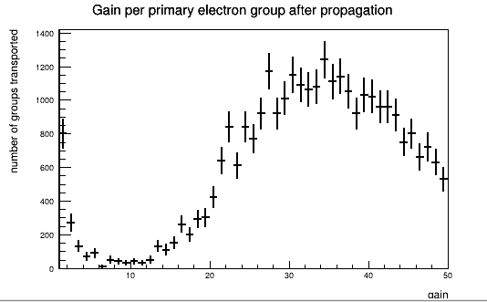
Looking at the distribution of gain per charge carrier I see that a lot of charge carriers have gain 1. My beam size is such the primary particle should always impact the sensor in the area of the gain layer and not in the edges, could this be due to deposited charges then propagated outside the gain layer area? Figure here:
thank you for your message. My first question would be, which Allpix version you are using. We did a few changes in the multiplication implementation in the past weeks, as a part of our version 3.0 release last week.
You are not the first to report gain values that are too low in comparison to measurement or other simulation, see e.g. Issues regarding the multiplication model - #25 by cferrero . We still do not know why that is the case, but first let me try to answer your questions. They will refer to the latest implementation of impact ionization that also comes with v3.0.
timestep parameter: The only dependency of the multiplication on the timestep should arise from variations of the electric field within individual steps. Hence, it makes sense to adapt the timestep parameter such, that the (spatial) step size is low enough to properly sample the implant region. You can easily get access to the spatial step size by switching on the DEBUG output for the TransientPropagation module (better do that for a single event only) as it prints out the step size. If you e.g. have a 1 um gain layer, you might want to go below 100 nm steps, which of course means that the timestep is rather small and the simulation time rather high. We have a few ideas on intermediate solutions to this dilemma (like a sub-sampling of the gain per step), but haven’t implemented this due to time constraints on our side. Please feel free to contribute if you have an idea on how to improve this.
To our experience, a level of 5 - 10 is a good setting for low-gain detectors, as this requires hole multiplication and typically the hole multiplication probability is comparatively low. To be sure, I would advise you to probe it by comparing the gain for a few different values, but my feeling is that the impact is low. We implemented this rather to prevent infinite multiplication loops, as we currently do not have any mechanisms that would introduce a quenching of such a behaviour.
The drawback is of course the precision of your simulation. In plain words, with more groups (less carriers per group) you increase statistics on stochastic processes (multiplication, diffusion). The way your simulation is set up (max_step_length=1um in deposition and charge_per_step=1000 in propagation, all charge carriers (roughly 80 per step) of one G4 step will be propagated together. Hence, if you e.g. have a particle traversing the sensor perpendicularly, you get in total 100 groups (50 e groups + 50 h groups) being propagated. To get representative results I would advise to reduce the charge_per_step, and in a 50 um thick sensor probably also the max_step_length parameter. One hint: what you will e.g. see in the pulsegraphs of the PulseTransfer module is that there is a strong oscillation in the beginning of the signal, which arises from this strong quantisation. This might be an interesting marker to look at.
As I do not know the layout of your sensor, this is honestly hard to tell. Did you verify that the beam particles don’t hit the sensor outside the gain layer? How deeply buried is the gain layer in your geometry? Could this be charge carriers that actually do not propagate through the gain layer?
One more thing I noticed in your configuration file: if you are using v3.0 or the latest master branch, the parameter multiplication_probability_based is not used anymore, as we dropped the non-stochastic approach.
All the above will help to make the simulation more physical. However, despite the change in version, I don’t expect a drastic influence on the gain. However, we would be grateful for feedback on this once you tuned the simulation a bit. As a short note on simulation vs expectations: we verified the mechanism by applying a constant gain in a geometrically precisely defined gain layer and the results matched the theoretical expectation well. Hence, we’re currently uncertain about what causes the discrepancy between simulation and measurement.
Thanks a lot for the very detailed explanation, this was super useful!
I tried your suggestions:
I’m indeed using the latest master branch version
regarding the timestep, 0.5ps allows me to have a 50nm spacial step size that should be sufficient to sample the 1um gain layer if I understand well. The simulation is indeed quite slow, but I have no suggestion on how to improve that I’m afraid.
I solved the problem of those events with gain 1, indeed they were not traversing the gain layer due to a bug in my setup, sorry for the confusion here
I changed the other parameters as suggested, however the gain distribution is still around 5-6 as you expected. On this mismatch I have to say that it could also be simply that the electric field I have it is not matching properly the one of the data I’m trying to compare. In any case thanks again for the suggestions!
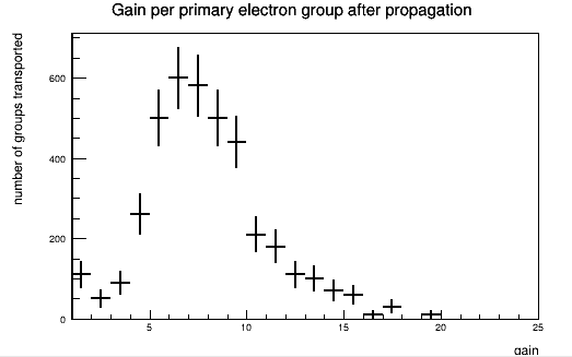
I was wondering what this bug in your setup was, @andrea_visibile ? For my simulations I get the following distributions with also a lot of electrons with gain 1. I am unsure if this is what I should expect, as @pschutze mentioned that the gain should have more of a exp^(-x) shape.
Perhaps I made the same mistake you did .
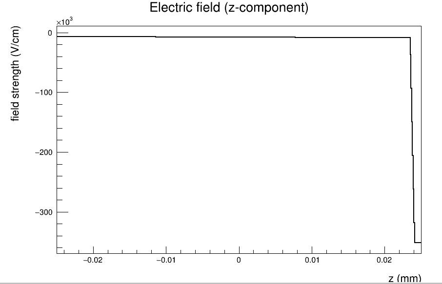
I am using my own implementation of a gain layered electric field, which has this shape:
in my case this was due to a mistake I made in dealing with the electric field of the TCAD map I’m using, leading to areas of the sensor (in x and y) where I should have had the gain layer and there was not instead. I guess this is very specific and probably not what is happening in your case.
thanks for sharing your insights!
Concerning the exp(-x) shape, I could imagine that we’re running into the central limit theorem here: if you propagate individual electrons, the probability of obtaining low gain values is still rather high. However, when you start grouping charge carriers (which you do by setting group_photons = 10 and not setting charge_per_step (default: 10) in the propagation) you start averaging out the gain of individual electrons, as we fill the histogram with final_charge_of_group / initial_charge_of_group. Hence you suppress low gains and move towards a normal distribution. In addition, the larger the gain, the lower the probability of low gains, obviously A good test would be to propagate single charge carriers and see how the distribution changes.
I would argue that the fraction of electrons with gain 1 is rather low, though not negligible. It would be interesting to follow up on this. My strong suspicion is that we are dealing with charge carriers that are generated very close to the sensor surface, such that they only do a very short step in the gain layer and have a reduced probability of multiplication. You could e.g. verify that by scanning the charge carrier deposition position via the DepositionPointCharge module.
I’d be happy to hear back in case you have new findings - this also helps us to gain (haha) experience on this matter.
Yes indeed, I noticed later that the problem was in the group_photons parameter. I am now using buckets of 1 and I get a nice exp(-x) function for gain.
You are right, maybe the problem is with the charges already in the gain layer, resulting an excess of charges with gain 1. That could explain the shape of the first histograms I sent
that sounds good. Don’t get me wrong, there’s nothing wrong with using the group_photons and with not getting an exp(-x) distribution, that’s just physics convolved with math
Getting back to the gain-1 electrons: I implemented graphs showing the average gain of a carrier as a function of creation depth and x/y, maybe that would be handy for you. It’s still a merge request, but if you’re curious you can check out my branch for that or look at the code.
Dear @andrea_visibile ,
I find a lot useful in your answer, thanks a lot!
I also have trouble in propagation progress. I use linear type electric field, and I also think the main problem is the electric filed. Could you tell me how to get a proper electric field?
Dear Nora,
in our case we’re using the output of a tcad simulation imported to allpix. However, we recently came to the conclusion that the electric field was fine and using another gain simulation model was enough to get a good comparison with our data.
in my case the okuto_optimised model works best, I guess cause the value of the parameters have also been optimised on lgads data with an electric field similar to the one I have, while before I was using the okuto or massey models. My understanding of these parametric models is that they work in a very specific subset of cases/ they’re not very flexible…
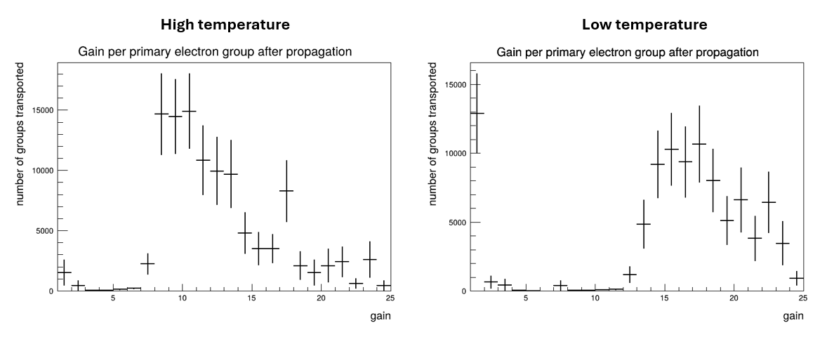
I think this thread is the right place for this question. I’m simulating the behaviour of LGAD sensors as a function of operational temperature. Everything seems to be working fine, but I’m having trouble with the gain histogram showing the number of transported groups: it’s being cropped at 25.
For high temperatures, that range is enough (as shown in the first figure). But at lower temperatures, I suspect I’m losing information, as the second plot suggests. Is there a way to expand the x-axis of this histogram?
one way is to change the axis in the code, but I would strongly recommend not use these auto-generated histograms for the analysis of your simulation, but to store the desired objects e.g. to a ROOT file using the ROOTObjectWriter and then to use your own analysis macro for generating the plots exactly as you need them.
There are some examples (in C++ and Python) in the repository: