Disappearing charge carriers, missing collected charge carriers, and too wide charge clouds,

Hi all,

This is going to be a bit long, and is separated into 3 parts.

I am simulating a detector, similar in geometry to the one simulated here by Sundberg et al.: 1-μm spatial resolution in silicon photon-counting CT detectors, and I have noticed some irregularities.
(Full .conf file is at the bottom)

Irregularity 1: disappearing charge carriers

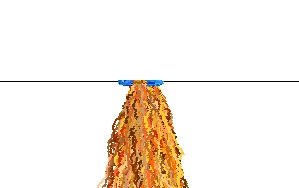
When generating an animation of the charge propagation, I noticed some of the charge carriers disappearing, as can be seen in the image below from the plot from TransientPropagation of the same event, where two of the charge carriers (on the right side) have disappeared on the way down to the backside electrode. Yes I have checked that the integration time is long enough (140ns), and the charge carriers disappears at around 20ns into the propagation according to the gif.


So my question is then, why does this happen?

Irregularity 2: Incomplete charge carrier collection.

This may be connected to irregularity 1, but there seems to be incomplete charge collection, which can be between a few percent, to 20 percent, for example with 20% discrepancy:

|10:31:00.740|    (INFO) (Event 7) [R:DepositionGeant4] Deposited 4918 charges in sensor of detector detector4
|10:31:03.502|    (INFO) (Event 7) [R:TransientPropagation:detector4] Propagated 4918 charges
                                                                      Recombined 0 charges during transport
                                                                      Trapped 0 charges during transport
|10:31:03.554|    (INFO) (Event 7) [R:PulseTransfer:detector4] Total charge induced on all pixels: -2023e

and for a few %:

|10:31:04.302|    (INFO) (Event 8) [R:DepositionGeant4] Deposited 4138 charges in sensor of detector detector2
|10:31:07.085|    (INFO) (Event 8) [R:TransientPropagation:detector2] Propagated 4138 charges
                                                                      Recombined 0 charges during transport
                                                                      Trapped 0 charges during transport
|10:31:07.134|    (INFO) (Event 8) [R:PulseTransfer:detector2] Total charge induced on all pixels: -1994e

I initially thought that it was a problem with the weighting potential, but then this should be fairly consistent if the number of charge carriers deposited is close to the same close to the same position, like above. However, this is seen for all energies, sometimes the collected charge carriers is close to the deposited, but always less, and sometimes it is a lot less.
So my question here then is: Where are the charges going?
To clarify, I am not using any recombination, trapping, or anything else. Here is the TransientPropagation config (full conf at bottom):

[TransientPropagation]
temperature = 293K
mobility_model = "jacoboni"
charge_per_step = 1
timestep = 0.1ns
integration_time =140ns
max_charge_groups = 0
distance = 2
output_plots = 1
output_linegraphs = true
output_plots_align_pixels = true
output_linegraphs_collected = true
output_linegraphs_recombined = true
output_linegraphs_trapped = true

Irregularity 3: too wide charge clouds

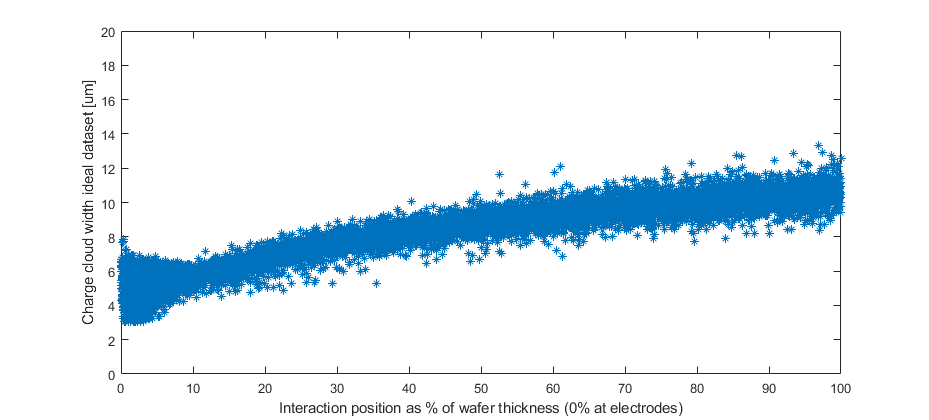
Similarly as in the article by Sundberg et al.: 1-μm spatial resolution in silicon photon-counting CT detectors, I am using a gaussian curve fit scheme to estimate the interaction position in one dimension (center of the gaussian), and using the standard deviation of the gaussian to find a power function fit to find the interaction position in the orthogonal direction (wafer thickness), from which we get the PSFs and MTFs for the two dimensions (orthogonal to the x-ray travel direction).
When performing the curve fit, we get good agreement in the wafer width direction, but the data diverge in its behaviour when looking at the set of standard deviations of all curve fits of the interactions.
In the figure below, one can see that there is a bell shape curving up when the interactions get closer to the collection electrodes (0% on the x-axis). This is, at least to me, counter intuitive, since the charges get less time to diffuse. Compare Figure 5a in the article by Sundberg. Note that most of the bell curve up-tick is from low energy interactions, but this could also be due to most of the compton interactions (the only ones considered here) are low energy.

To clarify, the pixel pitch is similar to the ~12um as in the article above in the width direction, and ~500um in the direction parallell to the x-ray path. The main difference is electrodes of ~1um compared to 10um used by Sundberg.
Further, the interactions are filtered such that only the ones where all charge is collected in one electrode row are kept. Further, here only the compton interactions are considered.
I then checked the number of electrodes that the charges spread to, which can be seen in the figure below, where the data points are colored by the total detected energy of all pixels in the event.
It doesn’t seem reasonable to see this kind of spread from compton interactions happening just a few microns from the electrodes.

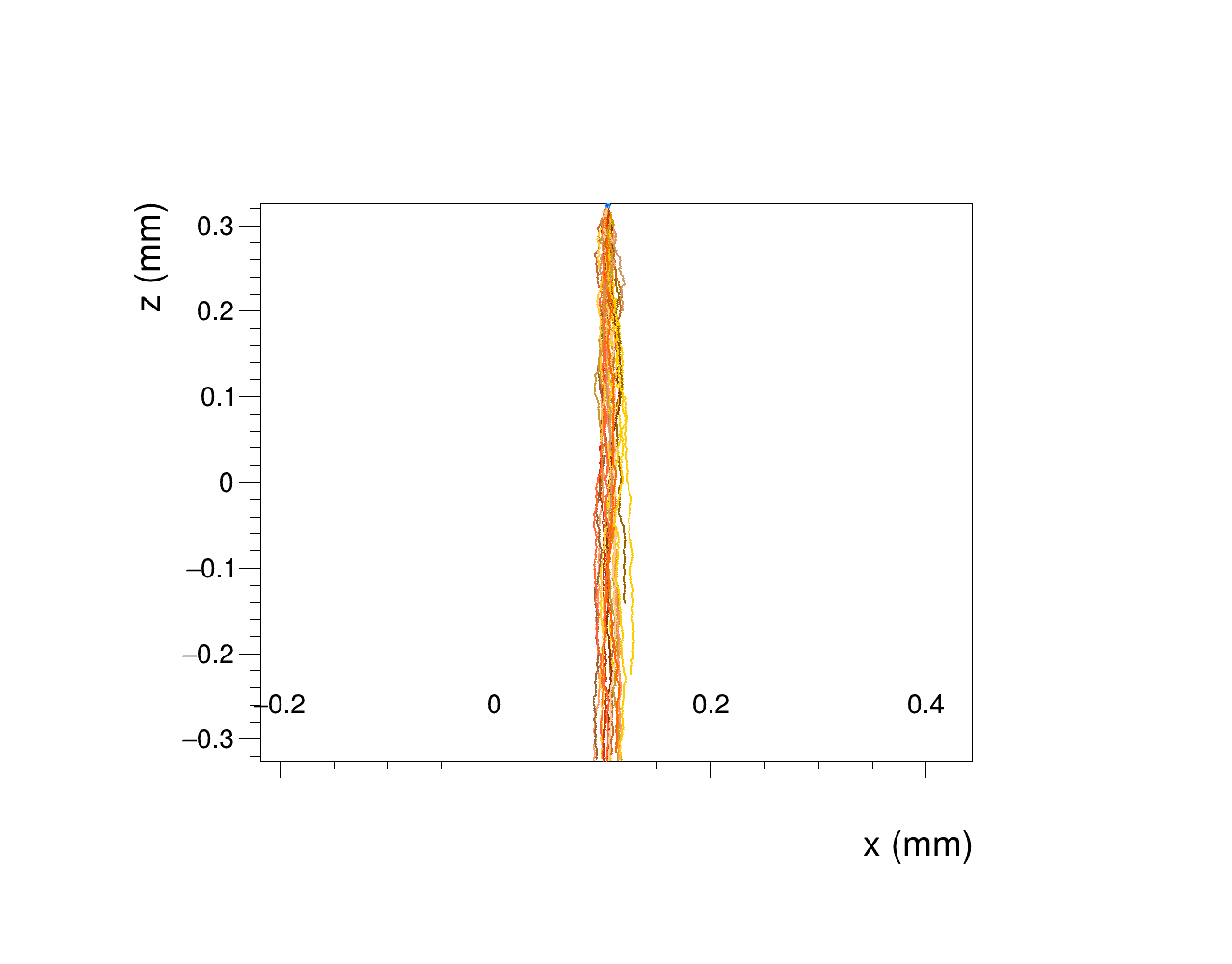
I also had a look at the line graphs from transient propagation, see the figures below. The first one shows an interaction where the electrons only spread a small amount, with the second one showing an interaction where the electrons seem to spread alot more than before. And the third one is zoomed in on a third interaction with a large spread. Apologies that it is difficult to see, haven’t found how to properly zoom in the 3D plots in TBrowser.


largespread

This is confusing me since there is no carrier-carrier interactions simulated.
My question(s) here then is: Where could this behaviour come from?, is it physical?, have I done something erroneous somewhere perhaps?

I did inspect the electric field mesh, but it seems to be correct as far as I can tell.

Taking any and all help and tips.

All the best,
Rickard

.conf file

[Allpix]
log_level = "INFO"
log_format = "DEFAULT"
detectors_file = "detector.conf"
number_of_events = 100
output_directory = "output"
[GeometryBuilderGeant4]
world_material = air

[DepositionGeant4]
physics_list = FTFP_BERT_PEN
record_all_tracks = true

source_type = "macro"
file_name = "xray_source_140kVp.mac" #140kVp source, filtered by Be, Al, H20 
number_of_particles = 1
max_step_length = 0.1um

[ElectricFieldReader]
model = "mesh"
file_name = electric_field.init"
field_mapping = "PIXEL_FULL"
log_level = "INFO"
output_plots = 1
output_plots_project = y
output_plots_projection_percentage = 0.5

[WeightingPotentialReader]
model = "mesh"
file_name = "weighting_potential.init"
field_mapping = "PIXEL_FULL"
log_level = "INFO"
output_plots = 1


[TransientPropagation]
temperature = 293K
mobility_model = "jacoboni"
charge_per_step = 1
timestep = 0.1ns
integration_time = 140ns
max_charge_groups = 0
distance = 2
output_plots = 1
output_linegraphs = true
output_plots_align_pixels = true
output_linegraphs_collected = true
output_linegraphs_recombined = true
output_linegraphs_trapped = true
#output_animations = true

[PulseTransfer]
output_plots = 1
output_pulsegraphs = true

#[Ignore]
[DefaultDigitizer]
electronics_noise = 0e
threshold = 0e
threshold_smearing = 0e
qdc_smearing = 0e


[ROOTObjectWriter]
# This is generally excluded, not now when debugging
#exclude = DepositedCharge, PropagatedCharge

Hi @rickard

this is indeed a lot to digest, but I think I have some leads for you.

1. irregularity

This we should look into, but I fear this is rather a plotting artifact and not necessarily connecteed with any of the below issues you mention. If you know which event this is happening in, you can re-run that single event (by setting the simulation seed and fast-forwarding with skip_events and number_of_events = 1) and set a DEBUG log level for the propagation module. You can then trace the individual groups through the silicon and see what happens to them

2. irregularity

In most cases I have seen where an incomplete induced current was detected, the problem is the interplay between the weighting potential and the defined electrode size. Explanation:

  • the induction algorithm stops, as soon as charge carriers enter the region defined as implant/electrode.
  • if this happens before the weighting potential has reached 1, there is an induced current missing
  • for transient simulations it therefore is of utmost importance to define the implant regions such, that they are inside (smaller than) the region where the weighting potential is 1.

Maybe check (or post) a close-up of your implant region of the weighting potential and e-field along with your sensor geometry file. (I know you had them somewhere in the forum already :grimacing: )

3. irregularity

I yet have to read the reference paper (and I fear I will not manage this year) but concerning the oddities you see I have a few comments even without that:

I then checked the number of electrodes that the charges spread to

You do not seem to apply any threshold to counting these electrodes, as long as they have seen any induced current. Depending on your weighting potential and your 5x5=25 pixels you calculate the induced current for, to me it does not sound entirely unreasonable to have such large “clusters”. Probably applying some 10e of threshold before counting would discard many of them

one shows an interaction where the electrons only spread a small amount, with the second one showing an interaction where the electrons seem to spread alot more than before

They impinge at different inter-pixel positions. Furthermore, this is only the projection of a 3D situation, so in the missing dimension there might also be an effect. Without looking at your electric field, but there seem to be some lateral components in it which spread charge carriers directly at the surface (between the electrodes, seems sensible to me) and with this initial spread of course the entire drift looks slightly different. If you look at the final spread at the sensor backside, it isn’t actually that different.

Last note on this, I recommend using the Canali model over Jacoboni, the latter is just a review of the former (among others) and very likely contains a typo in the saturation velocity of electrons. I don’t expect the difference to be significant though.

Cheers,
Simon

Hi @simonspa,

Thank you for the very fast reply to my very messy post!

Irregularity 1

I will see when I get the time to debug this part. I am suspecting the plotting to be the culprit as well, but just in case I will try and check it fairly soon!

Irregularity 2

I can’t post the exact specifications, since it is still a work in progress. I can however describe the details of the fields.

E-field

The electric field is (now in the beginning) simulated by creating a silicon block in comsol and segmenting the surface into electrodes and setting them and the backside to their respective potentials, and solving using the electrostatic module in COMSOL.

W-potential

The weighting potential is simualted the same way, though solving the Laplace equation with the center electrode set to unity potential, and the rest and the backside electrodes set to 0 potential. The edges of the simulation volume is set to floating, but is about ~300um away from the center pixel in each direction.
For the weighting potential, I am not entirely sure what the boundary conditions are supposed to be, and I can’t seem to find any definite answer. So if anyone have any insight on the boundary conditions at the edges of the simulated volume for the weighting potential, I’m all ears!

Electrodes/Implants

Since I have not simulated any 3D geometry of the electrodes, there are also no implants used in the detector configuration.

I would then assume, given your comment, that since the weighting potential and the electric field coincide exactly that there may be some discrepancy between the induced charge and the propagated charge.
But would this really explain the discrepancy variance of between 1%-20% difference?

Irregularity 3

That’s correct, I am using the full/raw output. However, in post-processing I have also tried to set a threshold to filter out the ones that detect only a few charges. Unfortunately the same effect still persists afterwards.

The pixels are very asymmetric and are several hundred times longer than they are wide, so any effect in this dimension should not matter much in this case.

When plotting the field, I cannot see any laterial components except for between the pixels very close to the surface, all of the field lines are pretty vertical towards the electrodes until in the close region of the electrodes.

I will give it a try!

Last note

Our old simulation software is based on Penelope with charge carrier propagation on top, which is what was used by Sundberg in the article linked above.
When comparing the code between our old software and the how allpix works (given the docs), the main differences are the use of Geant4 in allpix, and the propagation method. Our old software use basic Euler forward, and allpix use 4th order RK. Other than that the Jacoboni model is the same. Could this change of propagation method change the results this drastically perhaps?

Thank you for all your help,
Rickard

Hi @rickard

based on Penelope with charge carrier propagation on top

This is THOR then? Does that simulation implement transient simulations or does it collect charge carriers and count them? In that case, a comparison (for starters) with GenericPropagation might be more adequate.

use basic Euler forward, and allpix use 4th order RK

That might of course male a difference, but I would not expect it to have a big impact in a relatively straight-forward field as in your case. Tableaus for reference here, Euler is just

\begin{array}
{c|c}
1 & 1 \\
\hline
 &   1 \\
\end{array}

(darn, no math mode here)

/Simon

Hi @simonspa,

The code is written by my research group, but use Penelope for the charge depositions and with charge propagation using the Jacoboni model. It also implements transient propagation and reads out the induced charge using the Shockley-Ramo theorem.

Since the approaches are so similar, is is very confusing why we are getting so differently behaved results…

Just to expand on it, so you don’t need to read the paper, my approach is the same as in Sundberg et. al, where I fit a Gaussian to the detected energies in the pixels from an event, retrieving the interaction position in one dimension as the position of the peak, and the width of the charge cloud as the standard deviation of the Gaussian fit.

In the figures at the bottom (top ones are both from Sundberg et. al) the fit is to the left, and a scatter plot of the resulting standard deviation from all of the Gaussian fits is shown. The figure at the bottom is the standard deviation from my simulations using a similar pixel size but using Allpix Squared instead.

Even though I am seeing a slight improvement when adding a lowest threshold to filter out the interactions/pixels with only a few e in them, this bell shape persists strongly. Adding a higher lowest threshold (~1keV) makes most of the bell shape disappear, but it still persists from some of the higher energy interactions.

I am currently trying to fix the missing induced charges. Perhaps this is somehow connected to that…

All the best,
Rickard

Hi @rickard

my gut feeling says “electric field”. Just for the sake of finding out where to continue looking, I would do the following:

  • Switch back to GenericPropagation
  • Use a linear electric field, no weighting potential
  • Repeat the same simulation and check the curve shape

Then start re-adding things, and we might get a better handle where things go awry.

/Simon

PS: I read the paper, quite interesting :slight_smile:

Hi again, @simonspa

Before I go back to a linear field, I wanted to check what happens when the electrodes are simulated as 3D volumes in the silicon.

  1. I solved for the weighting potential again, this time the electrodes are a 3D volume with the center one set to unity and the remaining ones set to 0, each with a size of 3um by 3um.
  2. I did the same with the electric field, leaving the electrodes 1um by 1um.
  3. In APSQ I then set the implants to frontsize with a size of 1.5um by 1.5um.

Doing this I see that the majority of the bell from the interactions close to the electrodes disappears in the ideal dataset, see below, and all of the bell shape disappears when adding a realistic threshold with noise (not pictured).

HOWEVER:
when I looks at the detected energy in an event, I still see about 2% of the events have a detected energy error of more than 10% when compared to the deposited energy.

Error = [(sum of detected energy in all pixels) - (deposited energy)]/(deposited energy)*100

The figure below shows the number of events on the y axis that have an error of larger than the value on the x-axis.
The left most shows the histogram of the energy error of the events. The middle one shows the number of events that have an error larger than x[%], and the right most shows the same but as a percentage of the


The first few points are:
Error >0%: 96.05%
Error >1%: 8.01%
Error >2%: 5.63%
Error >3%: 4.39%
Error >4%: 3.35%
Error >5%: 2.88%
Error >6%: 2.63%
Error >7%: 2.45%
Error >8%: 2.30%
Error >9%: 2.21%
Error >10%: 2.10%

So about 2% of the interactions have an error of more than 10%.

So to end it off here, my questions are:

1. Since we have a discretization of the fields, it is reasonable to have some error, biased towards the negative side, as in the figure above. But is it reasonable to are the error % we see here reasonable, or is there perhaps something more at play here?

2. Do you have any recommendations for how to size the electrodes in the E-field simulation, compared to the weighting potential simulation, and lastly the implant size in APSQ (relative to each other)?

3. The backside implant shouldn’t impact much, but is it the same as with the frontside implants: define size of the implant and APSQ clones it to all pixels?

Thank you for the quick replies!

All the best,
Rickard